Author name: Vikram Chiluka

Python Interpolation To Fill Missing Entries

Interpolation is a Python technique for estimating unknown data points between two known data points. While preprocessing data, interpolation is commonly used to fill in missing values in a dataframe or series.

Interpolation is also used in image processing to estimate pixel values using neighboring pixels when extending or expanding an image.

Interpolation is also used by financial analysts to forecast the financial future based on known datapoints from the past.

Interpolation is commonly employed when working with time-series data since we want to fill missing values with the preceding one or two values in time-series data. For example, if we are talking about temperature, we would always prefer to fill today’s temperature with the mean of the last two days rather than the mean of the month. Interpolation can also be used to calculate moving averages.

Pandas Dataframe has interpolate() method that can be used to fill in the missing entries in your data.

The dataframe.interpolate() function in Pandas is mostly used to fill NA values in a dataframe or series. However, this is a really powerful function for filling in the blanks. Rather than hard-coding the value, it employs various interpolation techniques to fill in the missing data.

Interpolation for Missing Values in Series Data

Creation of pandas. Series with missing values as shown below:

# Import pandas module as pd using the import keyword
import pandas as pd
# Import numpy module as np using the import keyword
import numpy as np
# Pass some random list as an argument to thr pd.Series() method
# and store it in another variable.(defining series)
k = pd.Series([2, 3, 1,  np.nan, 4, 5, 8])

1)Linear Interpolation:

Linear interpolation basically implies estimating a missing value by connecting dots in increasing order in a straight line. In a nutshell, it estimates the unknown value in the same ascending order as prior values. Interpolation’s default method is linear, thus we didn’t need to specify it when using it.

The value at the fourth index in the above code is nan. Use the following code to interpolate the data:

k.interpolate()

In the absence of a method specification, linear interpolation is used as default.

# Import pandas module as pd using the import keyword
import pandas as pd
# Import numpy module as np using the import keyword
import numpy as np
# Pass some random list as an argument to thr pd.Series() method
# and store it in another variable.(defining series)
k = pd.Series([2, 3, 1,  np.nan, 4, 5, 8])
# Apply interpolate() function to the above series to fill the
# missing values(nan).
k.interpolate()

Output:

0    2.0
1    3.0
2    1.0
3    2.5
4    4.0
5    5.0
6    8.0
dtype: float64

2)Polynomial Interpolation:

You must specify an order in Polynomial Interpolation. Polynomial interpolation fills missing values with the lowest degree possible that passes via existing data points. The polynomial interpolation curve is similar to the trigonometric sin curve or assumes the shape of a parabola.

Polynomial interpolation needs the specification of an order. Here we see the interpolating with order 2 this time.

k.interpolate(method='polynomial', order=2)
# Import pandas module as pd using the import keyword
import pandas as pd
# Import numpy module as np using the import keyword
import numpy as np
# Pass some random list as an argument to thr pd.Series() method
# and store it in another variable.(defining series)
k = pd.Series([2, 3, 1,  np.nan, 4, 5, 8])
# Apply interpolate() function to the above series by giving the method as 
# "polynomial" and order= 2 as the arguments to fill the missing values(nan).
k.interpolate(method='polynomial', order=2)

Output:

0    2.000000
1    3.000000
2    1.000000
3    1.921053
4    4.000000
5    5.000000
6    8.000000
dtype: float64

When you use polynomial interpolation with order 1, you get the same result as linear interpolation. This is due to the fact that a polynomial of degree 1 is linear.

3)Interpolation Via Padding

Interpolation via padding involves copying the value just preceding a missing item.

When utilizing padding interpolation, you must set a limit. The limit is the maximum number of nans that the function can fill consecutively.

So, if you’re working on a real-world project and want to fill missing values with previous values, you’ll need to establish a limit on the number of rows in the dataset.

k.interpolate(method='pad', limit=2)
# Import pandas module as pd using the import keyword
import pandas as pd
# Import numpy module as np using the import keyword
import numpy as np
# Pass some random list as an argument to thr pd.Series() method
# and store it in another variable.(defining series)
k = pd.Series([2, 3, 1,  np.nan, 4, 5, 8])
# Apply interpolate() function to the above series by giving the method as 
# "pad" and limit = 2 as the arguments to fill the missing values(nan).
# The limit= 2 is the maximum number of nans that the function 
# can fill consecutively.
k.interpolate(method='pad', limit=2)

Output:

0    2.0
1    3.0
2    1.0
3    1.0
4    4.0
5    5.0
6    8.0
dtype: float64

The value of the missing entry is the same as the value of the entry preceding it.

We set the limit to two, so let’s see what happens if three consecutive nans occur.

k = pd.Series([0, 1, np.nan, np.nan, np.nan, 3,4,5,7])
k.interpolate(method='pad', limit=2)

Output:

0    0.0
1    1.0
2    1.0
3    1.0
4    NaN
5    3.0
6    4.0
7    5.0
8    7.0
dtype: float64

Here, the third nan is unaltered.

Pandas DataFrames Interpolation

Interpolation can also be used to fill missing values in a Pandas Dataframe.

Example

Approach:

  • Import pandas module as pd using the import keyword.
  • Pass some random data(as dictionary) to the pd.DataFrame() function to create a dataframe.
  • Store it in a variable.
  • Print the above-given dataframe.
  • The Exit of the Program.

Below is the implementation:

# Import pandas module as pd using the import keyword
import pandas as pd
  
# Pass some random data(as dictionary) to the pd.DataFrame() function
# to create a dataframe.
# Store it in a variable.
rslt_datafrme = pd.DataFrame({"p":[11, 3, 2, None, 1],
                   "q":[None, 1, 26, 8, None],
                   "r":[14, 10, None, 9, 4],
                   "s":[18, 5, None, None, 2]})
  
# Print the above given dataframe
print(rslt_datafrme)

Output:

      p     q     r     s
0  11.0   NaN  14.0  18.0
1   3.0   1.0  10.0   5.0
2   2.0  26.0   NaN   NaN
3   NaN   8.0   9.0   NaN
4   1.0   NaN   4.0   2.0

Pandas Dataframe Linear Interpolation

Do as given below to apply linear interpolation to the dataframe:

rslt_datafrme.interpolate()
# Import pandas module as pd using the import keyword
import pandas as pd
  
# Pass some random data(as dictionary) to the pd.DataFrame() function
# to create a dataframe.
# Store it in another variable.
rslt_datafrme = pd.DataFrame({"p":[11, 3, 2, None, 1],
                   "q":[None, 1, 26, 8, None],
                   "r":[14, 10, None, 9, 4],
                   "s":[18, 5, None, None, 2]})
  
# Apply interpolate() function to the above dataframe
rslt_datafrme.interpolate()

Output:

pqrs
011.0NaN14.018.0
13.01.010.05.0
22.026.09.54.0
31.58.09.03.0
41.08.04.02.0

In the above example, the first value below the ‘p’ column is still nan as there is no known data point before it for interpolation.

Individual columns of a dataframe can also be interpolated.

rslt_datafrme['r'].interpolate()
# Import pandas module as pd using the import keyword
import pandas as pd
  
# Pass some random data(as dictionary) to the pd.DataFrame() function
# to create a dataframe.
# Store it in another variable.
rslt_datafrme = pd.DataFrame({"p":[11, 3, 2, None, 1],
                   "q":[None, 1, 26, 8, None],
                   "r":[14, 10, None, 9, 4],
                   "s":[18, 5, None, None, 2]})
  
# Apply interpolate() function to the 'r' column of the above dataframe
rslt_datafrme['r'].interpolate()

Output:

0    14.0
1    10.0
2     9.5
3     9.0
4     4.0
Name: r, dtype: float64

Interpolation Via Padding

# Apply interpolate() function to the above dataframe by giving the method as 
"pad" and limit = 2 as the arguments to fill the missing values(nan). 

rslt_datafrme.interpolate(method='pad', limit=2)
# Import pandas module as pd using the import keyword
import pandas as pd
  
# Pass some random data(as dictionary) to the pd.DataFrame() function
# to create a dataframe.
# Store it in another variable.
rslt_datafrme = pd.DataFrame({"p":[11, 3, 2, None, 1],
                   "q":[None, 1, 26, 8, None],
                   "r":[14, 10, None, 9, 4],
                   "s":[18, 5, None, None, 2]})
  
# Apply interpolate() function to the above dataframe by giving the method as 
# "pad" and limit = 2 as the arguments to fill the missing values(nan).
rslt_datafrme.interpolate(method='pad', limit=2)

Output:

pqrs
011.0NaN14.018.0
13.01.010.05.0
22.026.010.05.0
32.08.09.05.0
41.08.04.02.0


Python Interpolation To Fill Missing Entries Read More »

Python Program for Calculating Summary Statistics

To calculate summary statistics in Python, use the pandas.describe() function. The describe() method can be used on both numeric and object data, such as strings or timestamps.

The result for the two will differ in terms of fields.

For numerical data, the outcome will be as follows:

  • count
  • mean
  • standard deviation
  • minimum
  • maximum
  • 25 percentile
  • 50 percentile
  • 75 percentiles

For Objects, the outcome will be as follows:

  • count
  • top
  • unique
  • freq

On DataFrame, a huge number of methods collectively generate descriptive statistics and other related activities. The majority of these are aggregations, such as sum() and mean(), although some, such as sumsum(), produce an object of the same size. In general, these methods, like ndarray.{sum, std,…}, accept an axis argument, but the axis can be supplied by name or integer.

Using Python’s describe() function, compute Summary Statistics

Let us now have a look at how to calculate summary statistics for object and numerical data by using the describe() method.

1)Calculation of Summary Statistics for Numerical data:

Approach:

  • Import pandas module using the import keyword.
  • Give the list as static input and store it in a variable.
  • Pass the given list argument to the pandas.series() function and store it in another variable. (defining series)
  • Apply describe() function to the above series to get the summary statistics for the given series.
  • The Exit of the Program.

Below is the implementation:

# Import pandas module using the import keyword
import pandas
# Give the list as static input and store it in a variable.
gvn_lst = [9, 5, 8, 2, 1]
# Pass the given list as an argument to the pandas.series() function and store it in
# another variable.(defining series)
rslt_seris = pandas.Series(gvn_lst)
# Apply describe() function to the above series to get the summary statistics
# for the given series.
rslt_seris.describe()

Output:

count    5.000000
mean     5.000000
std      3.535534
min      1.000000
25%      2.000000
50%      5.000000
75%      8.000000
max      9.000000
dtype: float64

Here each value has a definition. They are:

count: It is the number of total entries

mean: It is the mean of all the entries

std: It is the standard deviation of all the entries.

min: It is the minimum value of all the entries.

25%: It is the 25 percentile mark

50%: It is the 50 percentile mark i.e, median

75%: It is the 75 percentile mark

max: It is the maximum value of all the entries.

2)Calculation of Summary Statistics for Object data:

Approach:

  • Import pandas module using the import keyword.
  • Give the list of characters as static input and store it in a variable.
  • Pass the given list argument to the pandas.series() function and store it in another variable. (defining series)
  • Apply describe() function to the above series to get the summary statistics for the given series.
  • The Exit of the Program.

Below is the implementation:

# Import pandas module using the import keyword
import pandas
# Give the list of characters as static input and store it in a variable.
gvn_lst = ['p', 'e', 'r', 'g', 'e', 'p', 'e']
# Pass the given list as an argument to the pandas.series() function and store it in
# another variable.(defining series)
rslt_seris = pandas.Series(gvn_lst)
# Apply describe() function to the above series to get the summary statistics
# for the given series.
rslt_seris.describe()

Output:

count     7
unique    4
top       e
freq      3
dtype: object

Where

count: It is the number of total entries

unique: It is the total number of unique/distinct entries.

top: It is the value that occurred most frequently

freq: It is the frequency of the most frequent entry i.e here ‘e’ occurred 3 times hence its freq is 3.

Calculation of Summary Statistics for Huge dataset:

Importing the Dataset first and applying the describe() method to get Summary Statistics

Let us take an example of a cereal dataset

Import the dataset into a Pandas Dataframe.

Approach:

  • Import pandas module using the import keyword.
  • Import dataset using read_csv() function by passing the dataset name as an argument to it.
  • Store it in a variable.
  • Apply describe() method to the above-given dataset to get the Summary Statistics of the dataset.
  • The Exit of the Program.

Below is the implementation:

# Import pandas module as pd using the import keyword
import pandas as pd
# Import dataset using read_csv() function by passing the dataset name as
# an argument to it.
# Store it in a variable.
cereal_dataset = pd.read_csv('cereal.csv')
# Apply describe() method to the above-given dataset to get the Summary Statistics
# of the dataset.
cereal_dataset.describe()

Output:

caloriesproteinfatsodiumfibercarbosugarspotassvitaminsshelfweightcupsrating
count77.00000077.00000077.00000077.00000077.00000077.00000077.00000077.00000077.00000077.00000077.00000077.00000077.000000
mean106.8831172.5454551.012987159.6753252.15194814.5974036.92207896.07792228.2467532.2077921.0296100.82103942.665705
std19.4841191.0947901.00647383.8322952.3833644.2789564.44488571.28681322.3425230.8325240.1504770.23271614.047289
min50.0000001.0000000.0000000.0000000.000000-1.000000-1.000000-1.0000000.0000001.0000000.5000000.25000018.042851
25%100.0000002.0000000.000000130.0000001.00000012.0000003.00000040.00000025.0000001.0000001.0000000.67000033.174094
50%110.0000003.0000001.000000180.0000002.00000014.0000007.00000090.00000025.0000002.0000001.0000000.75000040.400208
75%110.0000003.0000002.000000210.0000003.00000017.00000011.000000120.00000025.0000003.0000001.0000001.00000050.828392
max160.0000006.0000005.000000320.00000014.00000023.00000015.000000330.000000100.0000003.0000001.5000001.50000093.704912

The result includes summary statistics for all of the columns in our dataset.

Calculation of Summary Statistics for timestamp series:

The describe() method is also used to obtain summary statistics for a timestamp series.

Approach:

  • Import pandas module using the import keyword.
  • Import datetime module using the import keyword.
  • Import numpy module as np using the import keyword
  • Give the timestamp as static input using the np.datetime64() function.
  • Store it in a variable.
  • Pass the given timestamp as an argument to the pandas.series() function and store it in another variable (defining series).
  • Apply describe() function to the above series to get the summary statistics for the given series.
  • The Exit of the Program.

Below is the implementation:

# Import pandas module using the import keyword
import pandas
# Import datetime module using the import keyword
import datetime
# Import numpy module as np using the import keyword
import numpy as np
# Give the timestamp as static input using the np.datetime64() function
# Store it in a variable.
gvn_timestmp = [np.datetime64("2005-04-03"), np.datetime64(
    "2008-05-01"), np.datetime64("2008-05-01"), np.datetime64("2003-01-07")]
# Pass the given timestamp as an argument to the pandas.series() function and
# store it in another variable.(defining series)
rslt_seris = pandas.Series(gvn_timestmp)
# Apply describe() function to the above series to get the summary statistics
# for the given series.
rslt_seris.describe()

Output:

count                       4
unique                      3
top       2008-05-01 00:00:00
freq                        2
first     2003-01-07 00:00:00
last      2008-05-01 00:00:00
dtype: object

You can also tell describe() method to treat dateTime as a numeric value. The result will be displayed in a way similar to that of numerical data. In the DateTime format, you can get the mean, median, 25th percentile, and 75th percentile.

rslt_seris.describe(datetime_is_numeric=True)
# Import pandas module using the import keyword
import pandas
# Import datetime module using the import keyword
import datetime
# Import numpy module as np using the import keyword
import numpy as np
# Give the timestamp as static input using the np.datetime64() function
# Store it in a variable.
gvn_timestmp = [np.datetime64("2005-04-03"), np.datetime64(
    "2008-05-01"), np.datetime64("2008-05-01"), np.datetime64("2003-01-07")]
# Pass the given timestamp as an argument to the pandas.series() function and
# store it in another variable.(defining series)
rslt_seris = pandas.Series(gvn_timestmp)
# Apply describe() function to the above series to get the summary statistics
# for the given series.
rslt_seris.describe(datetime_is_numeric=True)

Output:

count                      4
mean     2006-03-26 18:00:00
min      2003-01-07 00:00:00
25%      2004-09-10 18:00:00
50%      2006-10-17 00:00:00
75%      2008-05-01 00:00:00
max      2008-05-01 00:00:00
dtype: object


Python Program for Calculating Summary Statistics Read More »

Python loc() Function: To Extract Values from a Dataset

Python loc() Function:

Python is made up of modules that provide built-in functions for dealing with and manipulating data values.

Pandas is an example of such a module.

The Pandas module allows us to manage enormous data sets including a massive amount of data for processing all at once.

This is where Python’s loc() method comes into play. The loc() function makes it simple to retrieve data values from a dataset.

The loc() function allows us to obtain the data values fitted in a specific row or column based on the index value given to the function.

Syntax:

pandas.DataFrame.loc[index label]

We must supply the index values for which we want the whole data set to be shown in the output.

The index label could be one of the following values:

  • Single label – for example: String
  • List of string
  • Slice objects with labels
  • List of an array of labels, etc.

Using the loc() function, we may extract a specific record from a dataset depending on the index label.

If the provided index is not present as a label it returns KeyError.

Example

# Import pandas module using the import keyword
import pandas as pd
# Pass the some random list of data given to the DataFrame() function and store it in a variable
gvn_data = pd.DataFrame([[110, 2, 25, 14], [100, 3, 22, 10], [115, 1, 27, 9], [90, 5, 12, 14]],
     index=['Almond Delight', 'Clusters', 'Corn Chex', 'Cocoa Puffs'],
     columns=['calories', 'vitamins', 'fats','carboydrates'])
# Print the above dataframe
print("The given input Dataframe: ")
print(gvn_data)

Output:

The given input Dataframe: 
                calories  vitamins  fats  carboydrates
Almond Delight       110         2    25            14
Clusters             100         3    22            10
Corn Chex            115         1    27             9
Cocoa Puffs           90         5    12            14

Extraction of a Row from the Given Dataframe

Get all of the data values linked with the index label ‘clusters’ as shown below:

print(gvn_data.loc['Clusters'])
# Import pandas module using the import keyword
import pandas as pd
# Pass the some random list of data given to the DataFrame() function and store it in a variable
gvn_data = pd.DataFrame([[110, 2, 25, 14], [100, 3, 22, 10], [115, 1, 27, 9], [90, 5, 12, 14]],
     index=['Almond Delight', 'Clusters', 'Corn Chex', 'Cocoa Puffs'],
     columns=['calories', 'vitamins', 'fats','carboydrates'])
# Get all of the data values linked with the index label 'Clusters' using the
# loc[] function and print it.
print(gvn_data.loc['Clusters'])

Output:

calories        100
vitamins          3
fats             22
carboydrates     10
Name: Clusters, dtype: int64

Extraction of Multiple Rows from the Given Dataframe

We cal also get the multiple rows from the given dataframe.

Get all of the data values linked with the index labels ‘clusters’,  ‘Almond Delight’ as shown below:

print(gvn_data.loc[['Clusters', 'Almond Delight']])
# Import pandas module using the import keyword
import pandas as pd
# Pass the some random list of data given to the DataFrame() function and store it in a variable
gvn_data = pd.DataFrame([[110, 2, 25, 14], [100, 3, 22, 10], [115, 1, 27, 9], [90, 5, 12, 14]],
     index=['Almond Delight', 'Clusters', 'Corn Chex', 'Cocoa Puffs'],
     columns=['calories', 'vitamins', 'fats','carboydrates'])
# Extracting multiple rows from the given dataframe.
# Get all of the data values linked with the index labels 'clusters',  'Almond Delight'
# using the loc[] function and print it.
print(gvn_data.loc[['Clusters', 'Almond Delight']])

Output:

                calories  vitamins  fats  carboydrates
Clusters             100         3    22            10
Almond Delight       110         2    25            14

Extraction of Range of Rows from the Given Dataframe

We can retrieve data values of the range of rows using the loc[] function and slicing operator as shown below:

print(gvn_data.loc['Clusters': 'Cocoa Puffs'])
# Import pandas module using the import keyword
import pandas as pd
# Pass the some random list of data given to the DataFrame() function and store it in a variable
gvn_data = pd.DataFrame([[110, 2, 25, 14], [100, 3, 22, 10], [115, 1, 27, 9], [90, 5, 12, 14]],
     index=['Almond Delight', 'Clusters', 'Corn Chex', 'Cocoa Puffs'],
     columns=['calories', 'vitamins', 'fats','carboydrates'])
# Extracting range of rows from the given dataframe.
# Get all of the data values linked with the index labels 'clusters' to 'Cocoa Puffs '
# using the loc[] function,slicing operator and print it.
print(gvn_data.loc['Clusters': 'Cocoa Puffs'])

Output:

             calories  vitamins  fats  carboydrates
Clusters          100         3    22            10
Corn Chex         115         1    27             9
Cocoa Puffs        90         5    12            14


Python loc() Function: To Extract Values from a Dataset Read More »

In Python, How do you subset a DataFrame?

In this article, we will go through numerous methods for subsetting a dataframe. If you are importing data into Python then you must be aware of Data Frames. A DataFrame is a two-dimensional data structure in which data is aligned in rows and columns in a tabular form.

We may do various operations on a DataFrame using the Pandas library. We can even construct and access a DataFrame subset in several formats.

subsetting:

The process of picking a set of desired rows and columns from a data frame is known as subsetting.

We have the following options to select:

  • All rows and only a few columns(limited columns)
  • All columns and only a few rows
  • A limited number of rows and columns

Subsetting a data frame is useful since it allows you to access only a portion of the data frame. When you wish to reduce the number of parameters in your data frame, this comes in helpful.

Let us take a cereal dataset as an example.

Importing and Getting first 5 rows of the Dataset

Import the dataset into a Pandas Dataframe.

Apply head() function to the above dataset to get the first 5 rows.

cereal_dataset.head()
# Import pandas module as pd using the import keyword
import pandas as pd
# Import dataset using read_csv() function by pasing the dataset name as
# an argument to it.
# Store it in a variable.
cereal_dataset = pd.read_csv('cereal.csv')
# Apply head() function to the above dataset to get the first 5 rows.
cereal_dataset.head()

Output:

namemfrtypecaloriesproteinfatsodiumfibercarbosugarspotassvitaminsshelfweightcupsrating
0100% BranNC704113010.05.062802531.00.3368.402973
1100% Natural BranQC12035152.08.08135031.01.0033.983679
2All-BranKC70412609.07.053202531.00.3359.425505
3All-Bran with Extra FiberKC504014014.08.003302531.00.5093.704912
4Almond DelightRC110222001.014.08-12531.00.7534.384843

Using the Indexing Operator, select a subset of a dataframe.

The Indexing Operator is simply another term for square brackets. Using just the square brackets, you can select columns, rows, or a combination of rows and columns.

1)Selection of Only Columns

Use the below line of code to choose a column using the indexing operator.

cereal_dataset['vitamins']

The above line of code selects the column with the label ‘vitamins’ and displays all row values associated with it.

# Import pandas module as pd using the import keyword
import pandas as pd
# Import dataset using read_csv() function by pasing the dataset name as
# an argument to it.
# Store it in a variable.
cereal_dataset = pd.read_csv('cereal.csv')
# Apply head() function to the above dataset to get the first 5 rows.
cereal_dataset.head()
# Get all the rows values corresponding to the 'vitamins' column in the 
# above given dataset
cereal_dataset['vitamins']

Output:

0     25
1      0
2     25
3     25
4     25
      ..
72    25
73    25
74    25
75    25
76    25
Name: vitamins, Length: 77, dtype: int64

Selection of Multiple Columns

Select multiple columns using the index Operator.
Get all the rows values corresponding to the ‘vitamins’, ‘fat’ columns in the above-given dataset
cereal_dataset[['vitamins', 'fat']]
# Import pandas module as pd using the import keyword
import pandas as pd
# Import dataset using read_csv() function by pasing the dataset name as
# an argument to it.
# Store it in a variable.
cereal_dataset = pd.read_csv('cereal.csv')
# Apply head() function to the above dataset to get the first 5 rows.
cereal_dataset.head()
# Select multiple columns using the index Operator.
# Get all the rows values corresponding to the 'vitamins','fat' columns in the 
# above given dataset
cereal_dataset[['vitamins', 'fat']]

Output:

vitaminsfat
0251
105
2251
3250
4252
72251
73251
74251
75251
76251

77 rows × 2 columns

It generates a separate data frame that is a subset of the original.

2)Selection of Rows

The indexing operator can be used to pick specific rows depending on specified conditions.

To pick rows with ‘vitamins’ greater than 50, use the code below:

vitmns_grtrthan50= cereal_dataset[cereal_dataset['vitamins']>50]
vitmns_grtrthan50

Output:

namemfrtypecaloriesproteinfatsodiumfibercarbosugarspotassvitaminsshelfweightcupsrating
38Just Right Crunchy NuggetsKC110211701.017.066010031.01.0036.523683
39Just Right Fruit & NutKC140311702.020.099510031.30.7536.471512
53Product 19KC100303201.020.034510031.01.0041.503540
69Total Corn FlakesGC110212000.021.033510031.01.0038.839746
70Total Raisin BranGC140311904.015.01423010031.51.0028.592785
71Total Whole GrainGC100312003.016.0311010031.01.0046.658844

Using Python.loc(), select a Subset of a dataframe.

The.loc indexer is a powerful tool for selecting rows and columns from a data frame. It can also be used to select both rows and columns at the same time.

Note: It’s vital to understand that.loc() function only works on the labels of rows and columns. Following that, we’ll look at.iloc(), which is based on a row and column index.

 1)Selection of a Row using loc():

Use the following code to choose a single row with.loc().

cereal_dataset.loc[2]
# Import pandas module as pd using the import keyword
import pandas as pd
# Import dataset using read_csv() function by pasing the dataset name as
# an argument to it.
# Store it in a variable.
cereal_dataset = pd.read_csv('cereal.csv')
# Get all the 2nd rows values in the above given dataset using the loc[] function
cereal_dataset.loc[2]

Output:

name        All-Bran
mfr                K
type               C
calories          70
protein            4
fat                1
sodium           260
fiber              9
carbo              7
sugars             5
potass           320
vitamins          25
shelf              3
weight             1
cups            0.33
rating       59.4255
Name: 2, dtype: object

 Selection of Multiple Rows using loc():

cereal_dataset.loc[[2,4,6]]
# Import pandas module as pd using the import keyword
import pandas as pd
# Import dataset using read_csv() function by pasing the dataset name as
# an argument to it.
# Store it in a variable.
cereal_dataset = pd.read_csv('cereal.csv')
# Retrieving Multiple rows data
# Get all the 2, 4, 6 rows values in the above given dataset using the loc[] function
cereal_dataset.loc[[2, 4, 6]]

Output:

namemfrtypecaloriesproteinfatsodiumfibercarbosugarspotassvitaminsshelfweightcupsrating
2All-BranKC70412609.07.053202531.00.3359.425505
4Almond DelightRC110222001.014.08-12531.00.7534.384843
6Apple JacksKC110201251.011.014302521.01.0033.174094

Getting Range of Rows:

We can get rows data by providing the range (lower and upper limits) using slicing and loc[] function.

cereal_dataset.loc[3:6]
# Import pandas module as pd using the import keyword
import pandas as pd
# Import dataset using read_csv() function by pasing the dataset name as
# an argument to it.
# Store it in a variable.
cereal_dataset = pd.read_csv('cereal.csv')
# Retrieving Multiple rows data
# Get 3 to 6 rows data by providing the range (lower and upper limits) 
# using slicing and loc[] function.
cereal_dataset.loc[3:6]

Output:

namemfrtypecaloriesproteinfatsodiumfibercarbosugarspotassvitaminsshelfweightcupsrating
3All-Bran with Extra FiberKC504014014.08.003302531.00.5093.704912
4Almond DelightRC110222001.014.08-12531.00.7534.384843
5Apple Cinnamon CheeriosGC110221801.510.510702511.00.7529.509541
6Apple JacksKC110201251.011.014302521.01.0033.174094

2)Selection of rows and columns using loc()

Use the below line of code to choose specific rows and columns from the given data frame:

cereal_dataset.loc[3:6,['vitamins',' fats']]
# Import pandas module as pd using the import keyword
import pandas as pd
# Import dataset using read_csv() function by pasing the dataset name as
# an argument to it.
# Store it in a variable.
cereal_dataset = pd.read_csv('cereal.csv')
# Retrieving Multiple rows data
# Get vitamins, fat columns from 3 to 6 rows by providing the range (lower and upper limits)
# and columns using slicing and loc[] function.
cereal_dataset.loc[3:6,['vitamins', 'fat']]

Output:

vitaminsfat
3250
4252
5252
6250

Using Python.iloc(), select a Subset of a dataframe.

The iloc() function stands for integer location. It is completely based on integer indexing for both rows and columns.

Using iloc saves you from having to write down the entire label for each row and column.

Use iloc() to choose a subset of rows and columns as shown below:

cereal_dataset.iloc[[1,4,5], [2, 6]]

The above code selects rows 1, 4, and 5, as well as columns 2 and 6.

# Import pandas module as pd using the import keyword
import pandas as pd
# Import dataset using read_csv() function by pasing the dataset name as
# an argument to it.
# Store it in a variable.
cereal_dataset = pd.read_csv('cereal.csv')
# Retrieving Multiple rows data
# Get rows 1, 4, and 5, as well as columns 2 and 6 using iloc[] function.
cereal_dataset.iloc[[1,4,5], [2, 6]]

Output:

typesodium
1C15
4C200
5C180

After replacing the labels with integers, you can use iloc() to pick rows or columns individually, much like loc().

In Python, How do you subset a DataFrame? Read More »

Python Program for Coefficient of Determination – R Squared Value

Before delving into the topic of Coefficient of Determination, it is important to grasp the importance of evaluating a machine learning model using error metrics.

To solve any model in the field of Data Science, the developer must first analyze the efficiency of the model before applying it to the dataset. The model is evaluated using specific error metrics. One such error metric is the coefficient of determination.

Coefficient of Determination:

The coefficient of determination, often known as the R2 score. It is used to evaluate the performance of a linear regression model.

It is the degree of variation in the output-dependent attribute that can be predicted based on the input independent variable (s). It is used to determine how effectively the model reproduces observed results, based on the ratio of total deviation of results explained by the model.

R square has a range between [0,1].

Formula

R2= 1- SSres / SStot

where.

SSres: SSres is the sum of the squares of the residual errors of the data model’s
SStot: The total sum of the errors is represented by SStot.

Note: The higher the R square value, the better the model and the outcomes.

R2 With Numpy

Example:

Approach:

  • Import numpy module using the import keyword.
  • Give the list of actual values as static input and store it in a variable.
  • Give the list of predicted values as static input and store it in another variable.
  • Pass the given actual, predicted lists as the arguments to the corrcoef() function to get the Correlation Matrix.
  • Slice the matrix with the indexes [0,1] to get the value of R, also known as the Coefficient of Correlation.
  • Store it in another variable.
  • Calculate the value of R**2(R square) and store it in another variable.
  • Print the value of R square.
  • The Exit of the Program.

Below is the implementation:

# Import numpy module using the import keyword
import numpy
# Give the list of actual values as static input and store it in a variable.
actul_vals = [5, 1, 7, 2, 4]
# Give the list of predicted values as static input and store it in another
# variable.
predctd_vals = [4, 1.5, 2.8, 3.7, 4.9]
# Pass the given actual, predicted lists as the arguments to the corrcoef()
# function to get the Correlation Matrix
correltn_matrx = numpy.corrcoef(actul_vals, predctd_vals)
# Slice the matrix with the indexes [0,1] to get the value of R, also known
# as the Coefficient of Correlation.
rsltcorretn = correltn_matrx[0, 1]
# Calculate the value of R**2(R square) and store it in another variable.
Rsqure = rsltcorretn**2
# Print the value of R square
print("The result value of R square = ",Rsqure)

Output:

The result value of R square = 0.09902230080299725

R2 With Sklearn Library

The Python sklearn module has an r2_score() function for calculating the coefficient of determination.

Example

Approach:

  • Import r2_score function from sklearn.metrics module using the import keyword.
  • Give the list of actual values as static input and store it in a variable.
  • Give the list of predicted values as static input and store it in another variable.
  • Pass the given actual, predicted lists as the arguments to the r2_score() function to get the value of the coefficient of determination(R square).
  • Print the value of R square(coefficient of determination).
  • The Exit of the Program.

Below is the implementation:

# Import r2_score function from sklearn.metrics module using the import keyword. 
from sklearn.metrics import r2_score 
# Give the list of actual values as static input and store it in a variable.
actul_vals = [5, 1, 7, 2, 4]
# Give the list of predicted values as static input and store it in another
# variable.
predctd_vals = [4, 1.5, 2.8, 3.7, 4.9]
# Pass the given actual, predicted lists as the arguments to the r2_score()
# function to get the value of the coefficient of determination(R square).
Rsqure = r2_score(actul_vals, predctd_vals)
# Print the value of R square(coefficient of determination)
print("The result value of R square = ",Rsqure)

Output:

The result value of R square = 0.009210526315789336

Python Program for Coefficient of Determination – R Squared Value Read More »

Python Program for sample() Function with Examples

When handling problems involving data prediction, we frequently encounter scenarios in which we must test the algorithm on a small set of data to evaluate the method’s accuracy.

This is where the Python sample() function comes into play.

For operations, we may use the sample() method to select a random sample from the available data. Though there are other strategies for sampling data, the sample() method is widely regarded as one of the most simple.

Python’s sample() method works with all sorts of iterables, including list, tuple, sets, dataframes, and so on. It selects data from the iterable at random from the user-specified number of data values.

sample() Function:

sample() is a built-in function of Python’s random module that returns a specific length list of items taken from a sequence, such as a list, tuple, string, or set. Used for random sampling Non-replacement.

Syntax:

random.sample(sequence, k)

Parameters:

sequence: It may be a list, tuple, string, or set, etc.

k: It is an Integer. This is the length of a sample.

Return Value:

Returns a new list of k elements selected from the sequence.

Examples:

1)For Lists

Approach:

  • Import sample() function from the random module using the import keyword.
  • Give the list as static input and store it in a variable.
  • Give the length of the sample as static input and store it in another variable.
  • Pass the given list, sample length as the arguments to the sample() method to get the given length(len_sampl) of random sample items from the list.
  • Store it in another variable.
  • Print the above result.
  • The Exit of the Program.

Below is the implementation:

# Import sample() function from the random module using the import keyword.
from random import sample
# Give the list as static input and store it in a variable.
gvn_lst = [24, 4, 5, 9, 2, 1]
# Give the length of the sample as static input and store it in another variable.
len_sampl = 3
# Pass the given list, sample length as the arguments to the sample() method
# to get given length(len_sampl) of random sample items from the list
# Store it in another variable.
rslt = sample(gvn_lst, len_sampl)
# Print the above result.
print("The", len_sampl, "random items from the given list are:")
print(rslt)

Output:

The 3 random items from the given list are:
[9, 24, 4]
2)For Sets

Approach:

  • Import sample() function from the random module using the import keyword.
  • Give the set as static input and store it in a variable.
  • Give the length of the sample as static input and store it in another variable.
  • Pass the given set, sample length as the arguments to the sample() method to get the given length(len_sampl) of random sample items from the set.
  • Store it in another variable.
  • Print the above result.
  • The Exit of the Program.

Below is the implementation:

# Import sample() function from random module using the import keyword.
from random import sample
# Give the set as static input and store it in a variable.
gvn_set = {2, 4, 7, 1, 3, 1, 4, 2}
# Give the length of sample as static input and store it in another variable.
len_sampl = 4
# Pass the given set, sample length as the arguments to the sample() method
# to get given length(len_sampl) of random sample items from the set
# Store it in another variable.
rslt = sample(gvn_set, len_sampl)
# Print the above result.
print("The", len_sampl, "random items from the given set are:")
print(rslt)

Output:

The 4 random items from the given set are:
[1, 4, 7, 2]
Exceptions & Errors While using the sample() Function

When working with the sample() function, we may see a ValueError exception. This exception is thrown if the sample length is greater than the length of the iterable.

For Example:

# Import sample() function from the random module using the import keyword.
from random import sample
# Give the list as static input and store it in a variable.
gvn_lst = [24, 4, 5, 9, 2, 1]
# Give the length of the sample as static input and store it in another variable.
len_sampl = 10
# Pass the given list, sample length as the arguments to the sample() method
# to get given length(len_sampl) of random sample items from the list
# Store it in another variable.
rslt = sample(gvn_lst, len_sampl)
# Print the above result.
print("The", len_sampl, "random items from the given list are:")
print(rslt)

Output:

Traceback (most recent call last):
  File "/home/f39024cad259bfac4456fa81ec86fb82.py", line 10, in <module>
    rslt = sample(gvn_lst, len_sampl)
  File "/usr/lib/python3.6/random.py", line 320, in sample
    raise ValueError("Sample larger than population or is negative")
ValueError: Sample larger than population or is negative


Python Program for sample() Function with Examples Read More »

In Python, How can you Plot and Customize a Pie Chart?

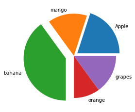
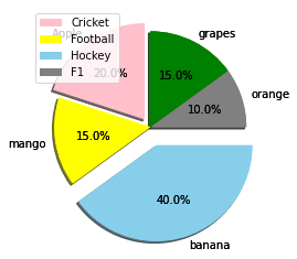
A pie chart is a circular statistical picture graph divided into slices to show numerical proportions. The arc length of each slice in a pie chart is proportionate to the quantity it represents.

The area of the wedge is defined by the length of the wedge’s arc. The area of a wedge represents the percentage of that part of the data in relation to the entire data set. Pie charts are widely used in corporate presentations to provide a brief review of topics such as sales, operations, survey data, and resources.

Pie charts are a common technique to display poll results.

Creating data

# Give some random list(fruits) as static input and store it in a variable.
fruit_lst = ["Apple", "mango", "banana", "orange", "grapes"]
# Give the percentage list as static input and store it in another variable.
gvn_percentges = [20, 15, 40, 10, 15]

How to Create a Pie Chart?

Matplotlib will be used to create a Pie-Chart.

In its pyplot module, the Matplotlib API offers a pie() method that generates a pie chart based on the data in an array.

Syntax:

matplotlib.pyplot.pie(data, explode=None, labels=None, colors=None, 
autopct=None, shadow=False)

Parameters

data: The array of data values to be plotted is represented by data, and the fractional area of each slice is represented by data/sum (data). If sum(data)<1 returns the fractional area directly, the resulting pie will have an empty wedge of size 1-sum (data).

labels: It is a list of string sequences that sets the label of each wedge.

colour: The colour attribute is used to give the colour of the wedge.

autopct: This is a string that is used to name each wedge with its numerical value.

shadow: The shadow is utilised to generate the shadow of the wedge.

To create a basic Pie-chart, we need labels and the values that go with those labels.

Example

Approach:

  • Import matplotlib.pyplot module as plt using the import keyword.
  • Give some random list(fruits) as static input and store it in a variable.
  • Give the percentage(size) list as static input and store it in another variable.
  • Get the subplots using the subplots function and assign it to two different variables.
  • Pass the given percentages(size)list, labels to the pie() function and apply it to the above axis (where labels is the fruit list).
  • Show the piechart using the show() function.
  • The Exit of the Program.

Below is the implementation:

# Import matplotlib.pyplot module as plt using the import keyword.
import matplotlib.pyplot as plt
# Give some random list(fruits) as static input and store it in a variable.
fruit_lst = ["Apple", "mango", "banana", "orange", "grapes"]
# Give the percentage list as static input and store it in another variable.
gvn_percentges = [20, 15, 40, 10, 15]
# Get the subplots using the subplots function and assign it to two different
# variables
figre, axis = plt.subplots()
# Pass the given percentages(size)list, labels to the pie() function
# and apply it to the above axis where labels is the fruit list.
axis.pie(gvn_percentges, labels=fruit_lst)
axis.axis('equal')
# Show the piechart using the show() function.
plt.show()

Output:


Customize a Pie Chart

A pie chart can be altered in a variety of ways. The startangle attribute spins the plot by the provided number of degrees in a counterclockwise direction on the pie chart’s x-axis. The shadow attribute accepts a boolean value; if true, the shadow appears below the rim of the pie. Wedges of the pie can be customized using wedgeprop, which accepts a Python dictionary as an argument and returns a list of name-value pairs specifying wedge attributes such as linewidth, edgecolor, and so on. A frame is drawn around the pie chart by setting frame=True axis. The percentages displayed on the wedges are controlled by autopct.

How to Make a slice pop-out?

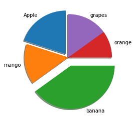
Using the explode option, you can make one or more pie-chart slices pop out.

To do this give an array with the explosion values. The explosion array provides the fraction of the radius by which to offset each slice.

Example

# Import matplotlib.pyplot module as plt using the import keyword.
import matplotlib.pyplot as plt
# Give some random list(fruits) as static input and store it in a variable.
fruit_lst = ["Apple", "mango", "banana", "orange", "grapes"]
# Give the percentage list as static input and store it in another variable.
gvn_percentges = [20, 15, 40, 10, 15]
#  Give the explode values as static input and store it in another variable.
explode_vals = (0.1, 0, 0.2, 0, 0)
# Get the subplots using the subplots function and assign it to two different
# variables
figre, axis = plt.subplots()
# Pass the given percentages(size)list, explode values, and labels to the pie() function
# and apply it to the above axis (where labels is the fruit list).
axis.pie(gvn_percentges, explode=explode_vals, labels=fruit_lst)
# Show the piechart using the show() function.
plt.show()

Output:

Rotating the Pie-chart

By defining a strartangle, you can rotate the pie-chart.

It rotates the start of the pie chart by the specified number of degrees counterclockwise from the x-axis.

Example

# Import matplotlib.pyplot module as plt using the import keyword.
import matplotlib.pyplot as plt
# Give some random list(fruits) as static input and store it in a variable.
fruit_lst = ["Apple", "mango", "banana", "orange", "grapes"]
# Give the percentage list as static input and store it in another variable.
gvn_percentges = [20, 15, 40, 10, 15]
#  Give the explode values as static input and store it in another variable.
explode_vals = (0.1, 0, 0.2, 0, 0)
# Get the subplots using the subplots function and assign it to two different
# variables
figre, axis = plt.subplots()
# Rotate the pie chart by giving the startangle.
axis.pie(gvn_percentges, explode=explode_vals, labels=fruit_lst,
        shadow=True, startangle=90)
# Show the piechart using the show() function.
plt.show()

Output:


To Display the percentages

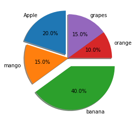
Display the percentages using the autopct.
# Import matplotlib.pyplot module as plt using the import keyword.
import matplotlib.pyplot as plt
# Give some random list(fruits) as static input and store it in a variable.
fruit_lst = ["Apple", "mango", "banana", "orange", "grapes"]
# Give the percentage list as static input and store it in another variable.
gvn_percentges = [20, 15, 40, 10, 15]
#  Give the explode values as static input and store it in another variable.
explode_vals = (0.1, 0, 0.2, 0, 0)
# Get the subplots using the subplots function and assign it to two different
# variables
figre, axis = plt.subplots()
# Display the percentages using the autopct
axis.pie(gvn_percentges, explode=explode_vals, labels=fruit_lst,
        autopct='%1.1f%%',shadow=True, startangle=90)
# Show the piechart using the show() function.
plt.show()

Output:


Color customization or Changing

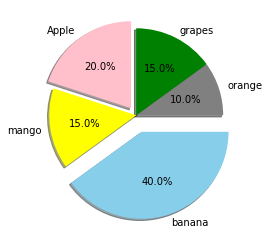
Matplotlib allows you to be creative and make your pie-chart as colorful as possible.

To modify the colors of your pie chart, give the colors list and apply those colors to the pie chart by giving it as an argument to the pie function().

# Import matplotlib.pyplot module as plt using the import keyword.
import matplotlib.pyplot as plt
# Give some random list(fruits) as static input and store it in a variable.
fruit_lst = ["Apple", "mango", "banana", "orange", "grapes"]
# Give the percentage list as static input and store it in another variable.
gvn_percentges = [20, 15, 40, 10, 15]
# Give the colors as static input and store it in another variable.
gvn_colors = ("pink", "yellow", "skyblue", "grey", "green")
# Give the explode values as static input and store it in another variable. 
explode_vals = (0.1, 0, 0.2, 0, 0)
figre, axis = plt.subplots()
# Applying the above given colors to the pie chart.
axis.pie(gvn_percentges, colors = gvn_colors, explode=explode_vals, labels=fruit_lst,
        autopct='%1.1f%%',shadow=True, startangle=90)
# Show the piechart using the show() function.
plt.show()

Output:


To Display the Color Codes

Along with your pie-chart, you can display a box containing the pie-color chart’s scheme. This is very beneficial if your pie chart has a lot of pieces.

Display the color codes using the legend() function.

Example

# Import matplotlib.pyplot module as plt using the import keyword.
import matplotlib.pyplot as plt
# Give some random list(fruits) as static input and store it in a variable.
fruit_lst = ["Apple", "mango", "banana", "orange", "grapes"]
# Give the percentage list as static input and store it in another variable.
gvn_percentges = [20, 15, 40, 10, 15]
# Give the colors as static input and store it in another variable.
gvn_colors = ("pink", "yellow", "skyblue", "grey", "green")
# Give the explode values as static input and store it in another variable. 
explode_vals = (0.1, 0, 0.2, 0, 0)
figre, axis = plt.subplots()
# Customized pie chart
axis.pie(gvn_percentges, colors = gvn_colors, explode=explode_vals, labels=fruit_lst,
        autopct='%1.1f%%',shadow=True, startangle=90)
patches, texts, auto = axis.pie(gvn_percentges, colors = gvn_colors, explode=explode_vals, labels=fruit_lst,
        autopct='%1.1f%%',shadow=True, startangle=90)
# Display the color codes using the legend() function
plt.legend(patches, labels, loc="best")
# Show the piechart using the show() function.
plt.show()

Output:


In Python, How can you Plot and Customize a Pie Chart? Read More »

In Python, How Do you Save a Dataframe as a csv File?

Pandas Module in Python:

Pandas is an open-source library based on the NumPy library. It enables users to perform effective data analysis, cleaning, and preparation. Pandas is fast, and it provides users with high performance and productivity.

The majority of the datasets you work with are referred to as DataFrames. DataFrames is a 2-Dimensional labeled Data Structure containing indexes for rows and columns, and each cell can store any form of value. DataFrames are simply Dictionary-based NumPy Arrays.

Creating a Dataframe

Approach:

  • Import os module using the import keyword.
  • Import pandas module using the import keyword.
  • Give some random list(fruits) as static input and store it in a variable.
  • Create a dictionary for the list of the above fruits and store it in another variable.
  • Pass the above fruit_dictnry as an argument to the pandas.DataFrame() function to create a dataframe for the above dictionary.
  • Print the above-obtained dataframe.
  • The Exit of the Program.

Below is the implementation:

# Import os module using the import keyword.
import os
# Import pandas module using the import keyword.
import pandas
# Give some random list(fruits) as static input and store it in a variable.
fruit_lst = ["Apple", "mango", "banana", "orange", "grapes", "Kiwi"]
# Create a dictionary for the above fruits list and store it in another variable.
fruit_dictnry = {'Types of Fruits': fruit_lst}
# Pass the above fruit_dictnry as an argument to the pandas.DataFrame() function
# to create a dataframe for the above dictionary.
rslt_dataframe = pandas.DataFrame(fruit_dictnry)
# Print the above obtained dataframe.
print(rslt_dataframe)

Output:

 Types of Fruits
0           Apple
1           mango
2          banana
3          orange
4          grapes
5            Kiwi

How to Save this Dataframe?

We frequently encounter circumstances in which we need to save large amounts of data generated by scraping or analysis in an easy, accesible  and readable form rather shareable form.

We can achieve this now by storing the data frame as a csv file.

dataframe.to_csv('filename.csv')

We can save a data frame as a CSV file using the pandas.to_csv() function. The file name must be passed as a parameter to the method.

Example

Approach:

  • Import os module using the import keyword.
  • Import pandas module using the import keyword.
  • Give some random list(fruits) as static input and store it in a variable.
  • Create a dictionary for the list of the above fruits and store it in another variable.
  • Pass the above fruit_dictnry as an argument to the pandas.DataFrame() function to create a dataframe for the above dictionary.
  • Save the above dataframe as a CSV file using the to_csv() function by passing some random file name as an argument that you want to save with.
  • Now the file will be saved as a csv file.
  • The Exit of the Program.

Below is the implementation:

from pandas.core.frame import DataFrame
# Import os module using the import keyword.
import os
# Import pandas module using the import keyword.
import pandas
# Give some random list(fruits) as static input and store it in a variable.
fruit_lst = ["Apple", "mango", "banana", "orange", "grapes", "Kiwi"]
# Create a dictionary for the above fruits list and store it in another variable.
fruit_dictnry = {'Types of Fruits': fruit_lst}
# Pass the above fruit_dictnry as an argument to the pandas.DataFrame() function
# to create a dataframe for the above dictionary.
rslt_dataframe = pandas.DataFrame(fruit_dictnry)
# Save the above dataframe as a CSV file using the to_csv() function by passing 
# some random file name as an argument that you want to save with.
rslt_dataframe.to_csv('fruits.csv')

Output:

Types of Fruits
0Apple
1mango
2banana
3orange
4grapes
5Kiwi


In Python, How Do you Save a Dataframe as a csv File? Read More »

Python Bar Plot: Visualization of Categorical Data

Data visualization allows us to analyze the data and examine the distribution of data in a pictorial way.

We may use BarPlot to visualize the distribution of categorical data variables. They depict a discrete value distribution. As a result, it reflects a comparison of category values.

The x-axis shows discrete values, whereas the y axis represents numerical values of comparison and vice versa.

BarPlot with Matplotlib

The Python matplotlib package includes a number of functions for plotting data and understanding the distribution of data values.

To construct a Bar plot with the matplotlib module, use the matplotlib.pyplot.bar() function.

Syntax:

matplotlib.pyplot.bar(x, height, width, bottom, align)

Parameters

x: The barplot’s scalar x-coordinates

height: It is the height of the bars to be plotted.

width: This is optional. It is the width of the bars to be plotted.

bottom: It is the vertical baseline.

align: This is optional. It is the type of bar plot alignment.

Example:

Approach:

  • Import matplotlib.pyplot module as plt using the import keyword.
  • Give some random list(gadgets) as static input and store it in a variable.
  • Give the other list(cost) as static input and store it in another variable.
  • Pass the given two lists as the arguments to the plt.bar() function to get the barplot of those lists.
  • Show the barplot of the given two lists using the show() function.
  • The Exit of the Program.

Below is the implementation:

# Import matplotlib.pyplot module using the import keyword.
import matplotlib.pyplot as plt
# Give some random list(gadgets) as static input and store it in a variable.
gadgets = ['mobile', 'fridge', 'washingmachine', 'tab', 'headphones']
# Give the other list(cost) as static input and store it in another variable.
costs = [15000, 20000, 18000, 5000, 2500]
# Pass the given two lists as the arguments to the plt.bar() function
# to get the barplot of those lists.
plt.bar(gadgets, costs)
# Show the barplot of the given two lists using the show() function.
plt.show()

Output:


BarPlot with Seaborn Library

Plots are mostly used to depict the relationship between variables. These variables can be entirely numerical or represent a category such as a group, class, or division. This article discusses categorical variables and how to visualize them using Python’s Seaborn package.

Seaborn, in addition to being a statistical plotting toolkit, includes various default datasets.

The Python Seaborn module is built on top of the Matplotlib module and provides us with some advanced functionalities for better data visualization.

Syntax:

seaborn.barplot(x, y)

Example:

Approach:

  • Import seaborn module using the import keyword.
  • Import matplotlib.pyplot module as plt using the import keyword.
  • Import dataset using read_csv() function by passing the dataset name as an argument to it.
  • Store it in a variable.
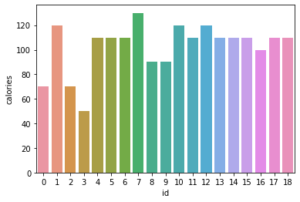
  • Pass the id, calories columns, and above dataset as the arguments to the seaborn.barplot() function to get the barplot of those.
  • Display the barplot of the using the show() function.
  • The Exit of the Program.

Below is the implementation:

# Import seaborn module using the import keyword.
import seaborn
# Import matplotlib.pyplot module as plt using the import keyword.
import matplotlib.pyplot as plt
# Import dataset using read_csv() function by passing the dataset name as
# an argument to it.
# Store it in a variable.
dummy_dataset = pd.read_csv('dummy_data.csv')
# Pass the id, calories columns and above dataset as the arguments to the 
# seaborn.barplot() function to get the barplot of those.
seaborn.barplot(x="id", y="calories", data=dummy_dataset)
# Display the barplot of the using the show() function.
plt.show()

Output:

Python Bar Plot: Visualization of Categorical Data Read More »

Python Program to Solve the Replace and Remove Problem

Replace and Remove problem:

The name of the problem is Replace and Remove Problem, and we will be replacing one specific character with a different string as well as removing a specific character from the user’s input.

So we know we need to replace one character with another string or set of characters and remove one character from the input. The two rules that we will abide by are as follows:

  1. Replace a with double d (dd)
  2. Remove any occurrence of b

Examples:

Example1:

Input:

Given String = "pythonarticlesbinarybooks"

Output:

Original String =  pythonarticlesbinarybooks
The result string =  pythonddrticlesinddryooks

Example2:

Input:

Given string ="haaabbcdcj"

Output:

Original String = haaabbcdcj
The result string = hddddddbcdcj

Program to Solve the Replace and Remove Problem in Python

Below are the ways to solve the replace and remove problem in Python:

Approach:

Convert the given string to list and Traverse the list check if the character is equal to ‘a’ if it is equal modify the list element with dd else check if the character is equal to ‘b’ then remove the element from the list.Join all elements of the list and print it.

Method #1: Using For loop (Static Input)

Approach:

  • Give the input string as static input and store it in a variable.
  • Convert the given string to a list using the list() function and store it in a variable.
  • Calculate the length of the list using the len() function and store it in a variable.
  • Loop till the length of the given list using the for loop.
  • Check if the list element at the iterator index is equal to a using the if conditional statement.
  • If it is true then replace the list element at iterator index with ‘dd’.
  • Loop in the above list using the For loop and in operator.
  • Check if the element is equal to ‘b’ using the if conditional statement.
  • If it is true then remove the element from the list using the remove() function.
  • After the end of for loop.
  • Convert the list to string using the join() function.
  • Print the string after joining the list elements.
  • The Exit of the Program.

Below is the implementation:

# Give the input string as static input and store it in a variable.
gvnstrng = 'pythonarticlesbinarybooks'
# Convert the given string to a list using the list() function and store it in a variable.
strnglist = list(gvnstrng)
# Calculate the length of the list using the len() function and store it in a variable.
lstlengt = len(strnglist)
# Loop till the length of the given list using the for loop.
for indx in range(lstlengt):
        # Check if the list element at the iterator index is equal to a
    # using the if conditional statement.
    if(strnglist[indx] == 'a'):
        # If it is true then replace the list element at iterator index with 'dd'.
        strnglist[indx] = 'dd'
# loop in the above list using the For loop and in operator
for ele in strnglist:
    # check if the element is equal to 'b' using the if conditional statement.
    if(ele == 'b'):
        # If it is true then remove the element from the list using the remove() function.
        strnglist.remove(ele)


# After the end of for loop.
# Convert the list to string using the join() function.
rststrng = ''.join(strnglist)
# Print the string after joining the list elements.
print('Original String = ', gvnstrng)
print('The result string = ', rststrng)

Output:

Original String =  pythonarticlesbinarybooks
The result string =  pythonddrticlesinddryooks

Method #2: Using For loop (User Input)

Approach:

  • Give the input string as user input using list(),map(),split(),int() functions and store it in a variable.
  • Convert the given string to a list using the list() function and store it in a variable.
  • Calculate the length of the list using the len() function and store it in a variable.
  • Loop till the length of the given list using the for loop.
  • Check if the list element at the iterator index is equal to a using the if conditional statement.
  • If it is true then replace the list element at iterator index with ‘dd’.
  • Loop in the above list using the For loop and in operator.
  • Check if the element is equal to ‘b’ using the if conditional statement.
  • If it is true then remove the element from the list using the remove() function.
  • After the end of for loop.
  • Convert the list to string using the join() function.
  • Print the string after joining the list elements.
  • The Exit of the Program.

Below is the implementation:

# Give the input string as user input using list(),map(),split(),int() functions and store it in a variable.
gvnstrng = input('Give some random string = ')
# Convert the given string to a list using the list() function and store it in a variable.
strnglist = list(gvnstrng)
# Calculate the length of the list using the len() function and store it in a variable.
lstlengt = len(strnglist)
# Loop till the length of the given list using the for loop.
for indx in range(lstlengt):
        # Check if the list element at the iterator index is equal to a
    # using the if conditional statement.
    if(strnglist[indx] == 'a'):
        # If it is true then replace the list element at iterator index with 'dd'.
        strnglist[indx] = 'dd'
# loop in the above list using the For loop and in operator
for ele in strnglist:
    # check if the element is equal to 'b' using the if conditional statement.
    if(ele == 'b'):
        # If it is true then remove the element from the list using the remove() function.
        strnglist.remove(ele)


# After the end of for loop.
# Convert the list to string using the join() function.
rststrng = ''.join(strnglist)
# Print the string after joining the list elements.
print('Original String = ', gvnstrng)
print('The result string = ', rststrng)

Output:

Give some random string = haaabbcdcj
Original String = haaabbcdcj
The result string = hddddddbcdcj

Python Program to Solve the Replace and Remove Problem Read More »