Author name: Prasanna

Python Programming – NumPy

Learn NumPy Library in Python – Complete Guide

Creating Numpy Arrays

  • Create NumPy Arrays from list, tuple, or list of lists
  • Create NumPy Arrays from a range of evenly spaced numbers using np.arrange().
  • Create NumPy Array of zeros (0’s) using np.zeros()
  • Create 1D / 2D NumPy Array filled with ones (1’s) using np.ones()
  • Create NumPy Array of different shapes & initialize with identical values using numpy.full()
  • Create NumPy Array with same sized samples over an interval in Python using numpy.linspace()
  • Create a NumPy Array of bool value.

Adding Elements in Numpy Array

Searching in Numpy Arrays

Get Metadata of Numpy Array

Selecting elements from Numpy Array

Modifying a Numpy Array

Converting NumPy Array to Other Data Structures

Numpy Array and File I/O

Verify Contents of Numpy Array

Counting Elements in Numpy Array

Advance Topics about Numpy Array

  • What is a Structured Numpy Array and how to create and sort it in Python?
  • numpy.zeros() & numpy.ones() | Create a numpy array of zeros or ones

Python Programming – NumPy

NUMPY

As discussed previously, simple one dimensional array operations can be executed using list, tuple etc. But carrying out multi-dimensional array operations using list is not easy. Python has an array module which provides methods for creating array, but they are slower to index than list. A good choice for carrying array operations is by using “NumPy” package.

NumPy is a Python package (licensed under the BSD license) which is helpful in scientific computing by providing multi-dimensional array object, various derived objects (such as masked arrays and matrices), and collection of routines for fast operations on arrays, including mathematical, logical, shape manipulation, sorting, basic linear algebra, basic statistical operations, and many more. At the core of the NumPy package, there is array object which encapsulates n-dimensional arrays of homogeneous data types. There are several important differences between the NumPy array and the standard Python sequence:

  • NumPy array has a fixed size at creation, unlike Python list (which can grow dynamically). Changing the size of a ndarray will create a new array and delete the original.
  • All elements in a NumPy array are required to be of the same data type.
  • NumPy array facilitates advanced mathematical and other types of operations on large numbers of data. Typically, such operations are executed more efficiently and with less code than is possible using Python’s built-in sequences.

History

NumPy is built on (and is a successor to) the successful “Numeric” package. Numeric was reasonably complete and stable, remains available, but is now obsolete. Numeric was originally written in 1995 largely by Jim Hugunin, while he was a graduate student at MIT. In 2001, Travis Oliphant along with Eric Jones and Pearu Peterson created “SciPy”, which had the the strenght of Numeric package along additional functionality. At about the same time as SciPy was being built, some Numeric users were hitting up against the limited capabilities of Numeric.

As a result, “numarray” (now obselete) was created by Perry Greenfield, Todd Miller, and RickWhite at the Space Science Telescope Institute as a replacement for Numeric. In early 2005, Travis Oliphant initiated an effort to bring the diverging community together under a common framework. The effort was paid off with the release of a new package Numpy (with version 0.9.2) in early 2006, which is an amalgam of the code base of Numeric with additional features of numarray. The NumPy name was christened from the unofficial name of “Numerical Python”.

Universal functions

NumPy provides familiar mathematical functions such as sin ( ), cos ( ), exp ( ), etc. In NumPy, these are called “universal functions”. Within NumPy, these functions operate element-wise on an array, producing an array as output.

>>> a=np . arange ( 3 ) 
>>> a 
array ( [ 0 , 1 , 2 ] ) 
>>> np . exp ( a ) 
array ( [ 1 . , 2 . 71828183 , 7 . 3890561 ] )
>>> np . sqrt ( a ) 
array ( [ 0 . , 1 . , 1 . 41421356 ] )

The Matrix Class

There is also a matrix class, which returns a matrix from an array-like object, or from a string of data. A matrix is a specialized 2-D array that retains its 2-D nature through operations.

>>> np . matrix ( [ [ 1 . 0 , 2 . 0 ] , [ 3 . 0 , 4 . 0 ] ] ) 
matrix ( [ [ 1 . , 2 . ] , 
[ 3 . , 4 . ] ] )
>>> a=np . matrix ( ' 1 . 0 2 . 0 ; 3 . 0 4 . 0 ' ) 
>>> a
matrix ( [ [ 1 . , 2 . ] , 
[ 3 . , 4 . ] ] )
>>> a . T                                                                           # Transpose of a matrix
matrix ( [ [ 1 . , 3 . ] ,
[ 2 . , 4 .] ] ) 
>>> x=np . matrix ( ' 5 . 0 7 . 0 ' )
>>> y=x.T
>>> y
matrix ( [ [ 5 . ] ,
[ 7 . ] ] )
>>> a*y                                                                          # Matrix multiplication
matrix ( [ [ 19 . ] ,
[ 43 . ] ] )
>>> a.I                                                                           # Inverse of a matrix
matrix ( [ [ -2 . , 1 . ] ,
[ 1 . 5 , -0 . 5 ] ] )

In this Page, We are Providing Python Programming – NumPy. Students can visit for more Detail and Explanation of Python Handwritten Notes Pdf.
Python Programming – NumPy Read More »

Python Programming – Basic Operations

In this Page, We are Providing Python Programming – Basic Operations. Students can visit for more Detail and Explanation of Python Handwritten Notes Pdf.

Python Programming – Basic Operations

Basic Operations

Arithmetic operations when applied on NumPy arrays, they are implemented element-wise.

>>> a=np . array ( [ 20 , 30 , 40 , 50 ] )
>>> b=np . arange ( 4 ) 
>>> c=a - b 
>>> c
array ( [ 20 , 29 , 38 , 47 ] )
>>> b**2
array ( [ 0 , 1 , 4 , 9 ] )
>>> a<39
array ( [ True , True , False , False ] , dtype=bool )

The product operator * operates element-wise in NumPy arrays. The matrix product can be performed using the dot ( ) function or creating matrix objects (refer section 7.8).

>>> a=np . array ( [ [ 1 , 1 ] ,
. . . [ 0 , 1 ] ] )
>>> b=np . array ( [ [ 2 , 0 ] ,
. . . [ 3 , 4 ] ] )
>>> a*b 
array ( [ [ 2 , 0 ] ,
[ 0 , 4 ] ] )
>>> np . dot ( a , b ) 
array ( [ [ 5 , 4 ] ,
[ 3 , 4 ] ] )

Some operations, such as +=, *=, etc., modifies an existing array, rather than creating a new array.

>>> a=np . array ( [ [ 1 , 2 ] ,                        # a is integer type
. . . [ 3 , 4 ] ] )
>>> b=np . array ( [ [ 1 . , 2 . ] ,                   # b is float type
. . . [ 3 . , 4 . ] ] )
>>> a*=2 
>>> a
array ( [ [ 2 , 4 ] ,
[ 6 , 8 ] ] )
>>> b+=a 
>>> b
array ( [ [ 3 . , 6 . ] ,
[ 9 . , 12 . ] ] )
>>> a+=b                                                  # b is converted to integer type
>>> a
array ( [ [ 5 , 10 ] ,
[ 15 , 20 ] ] )

When operating with arrays of different types, the type of the resulting array corresponds to the more general or precise one (a behavior known as “upcasting”).

>>> a=np . array ( [ 1 . 1 , 2 . 2 , 3 . 3 ] )
>>> a . dtype . name
' float64 ' 
>>> b=np . array ( [ 4 , 5 , 6 ] )
>>> b . dtype . name ' int32 '
>>> c=a+b 
>>> c
array 0( [ 5 . 1 , 7 . 2 , 9 . 3 ] )
>>> c . dtype . name ' float64 '

Many unary operations, such as computing the sum of all the elements in the array, are implemented as methods of the ndarray class .

>>> a=np . array ( [ [5 , 8 ] ,
. . . [ 3 , 6 ] ] )
>>> a . sum ( )
22
>>> a . min ( )
3
>>> a . max ( )
8

By default, these operations apply to the array as though it were a list of numbers, regardless of its shape. However, by specifying the axis parameter you can apply an operation along the specified axis of an array:

>>> a=np . arange ( 12 ) . reshape ( 3 , 4 )
>>> a
array ( [ [ 0 , 1 , 2 , 3 ] ,
[ 4 , 5 , 6 , 7 ] ,
[ 8 , 9 , 10 , 11 ] ] )
>>> a.sum(axis=0)                                             # Sum of each column
array ( [12, 15, 18, 21] )
>>> a.min(axis=1)                                             # Minimum of each now
array ( [ 0 , 4 , 8 ] )
>>> a . cumsum ( axis=1 )                                  # Cumulative sum along each now
array ( [ [ 0 , 1 , 3 , 6 ] ,
[ 4 , 9 , 15 , 22 ] ,
[ 8 , 17 , 27 , 38 ] ] )

Python Programming – Basic Operations Read More »

Python Programming – NumPy Array

In this Page, We are Providing Python Programming – Numpy Array. Students can visit for more Detail and Explanation of Python Handwritten Notes Pdf.

Python Programming – NumPy Array

NumPy array

NumPy’s main object is the homogeneous multi-dimensional array. It is a table of elements (usually numbers), all of the same type, indexed by a tuple of positive integers. In NumPy, array dimensions are called “axes”, and the number of axes is known as “rank”. For example, the coordinates of a point in 3D space [ 1, 2, 1 ] is an array of rank 1, because it has one axis and that axis has a length of 3. In the following example, the array has rank 2 (it is two-dimensional). The first dimension (axis) has a length of 2, the second dimension has a length of 3.

[ [ 1 . , 0 . , 0 . ] , 
[ 0 . , 1 . , 2 . ] ]

Some of the attributes of an ndarray object are:

ndarray . ndim
The number of axes (dimensions) or rank of the array.

ndarray . shape
The dimensions of the array. This is a tuple of integers indicating the size of the array in each dimension. For an array of n rows and m columns, shape will be (n, m). The length of the shape tuple is therefore the rank ndim.

ndarray.size
The total number of elements of the array. This is equal to the product of the elements of shape.

ndarray.dtype
An object describing the type of the elements in the array. One can create or specify dtype using standard Python type. Additionally, NumPy provides types of its own, numpy.int32, numpy. intl6, and numpy. f loat64 are some examples.

ndarray.itemsize
The size in bytes of each element of the array. For example, an array of elements of type float 6 4 has itemsize as 8 (=64/8), while one of type complex32 has itemsize as 4 (=32/8). It is equivalent to ndarray. dtype . itemsize.’


>>> import numpy as np
>>> a=np . array ( [ [ 0 , 1 , 2 , 3 , 4 ] ,
. . .                           [ 5 , 6 , 7 , 8 , 9 ] , 
. . .                           [ 10 , 11 , 12 , 13 , 14 ] ] )
. . . 
>>> type ( a )
<type ' numpy . ndarray ' > 
>>> a . shape 
( 3 , 5 )
>>> a . ndim 
2
>>> a.dtype 
dtype ( ' int32 ' )
>>> a . dtype . name
' int32 '
>>> a.itemsize 
4
>>> a . size 
15

Array creation

There are several ways to create NumPy array, one approach is from a regular Python list or tuple using the array () method. The type of the resulting array is deduced from the type of the elements in the sequences.

>>> import numpy as np 
>>> a=np.array ( [ 1 , 2 , 3 ] )
>>> a . dtype 
dtype ( ' int32 ' )
>>> b=np . array ( ( 1 . 2 , 3 . 4 , 5 . 6 ) )
>>> b. dtype 
dtype ( ' float64 ' )

A frequent error consists in calling array ( ) with multiple numeric arguments, rather than providing a single list or tuple of numbers as an argument.

>>> a=np . array ( 1 , 2 , 3 , 4 )      # WRONG
>>> a=np . array ( [ 1 , 2 , 3 , 4] )  # RIGHT

array ( ) transforms sequence of sequences into two-dimensional arrays, sequences of sequences of sequences into three-dimensional arrays, and so on.

>>> b=np . array ( [ ( 1 . 5 , 2 , 3 ) , ( 4 , 5 , 6 ) ] )
>>> b
array ( [ [ 1 . 5 , 2 . , 3 . ] ,
[ 4 . , 5 . , 6 . ] ] )

The type.of the array can also be explicitly specified at creation time:

>>> c=np . array ( [ [ 1 , 2 ] , [ 3 , 4 ] ] , dtype=np.complex)
>>> c
array ( [ [ 1 .+0 . j , 2 . + 0 . j ] ,
[ 3 . +0 . j , 4 . + 0 . j ] ] )

Often the elements of an array are initially unknown, but array size is known. Hence, NumPy offers several functions to create array with initial placeholder content. The function zeros ( ) create an array full of zeros, the function ones ( ) create an array full of ones, and the function empty ( ) create an array whose initial content is random. By default, the dtype of the created array is f loat6 4.

>>> np. zeros ( ( 3 , 4 ) )
array ( [ [ 0 . , 0 . , 0 . , 0 . ] ,
             [ 0 . , 0 . , 0 . , 0 . ] ,
             [ 0 . , o . , 0 . , 0 . ] ] )
>>> np . zeros [ 3 , 4] ) 
array ( [ [ 0 . , o . , o . , 0 . ] ,
           [ o . , o . , o . , 0 . ] ,
           [ o . , o . , o . , 0 . ] ] )
>>> np . ones ( ( 2 , 3 , 4 ) , dtype=np . int16 ) 
array ( [ [ [ 1 , 1 , 1 , 1 ] ,
           [ 1 , 1 , 1 ] ,
           [ 1 , 1 , 1 , 1] ] ,

           [ [ 1 , 1 , 1 , 1 ] ,
           [ 1 , 1 , 1 , 1 ] ,
           [ 1 , 1 , 1 , 1 ] ] ] , dtype=intl6 )
>>> np . empty ( ( 2 , 3 ) )
array ( [ [ 1 . 39069238e-309 , 1 . 39069238e-309 , 1 . 39069238e-309 ] ,
           [ 1 . 39069238e-309 , 1 . 39069238e-309 , 1 . 39069238e-309 ] ] )


To create sequences of numbers, NumPy provides a function arange ( ), analogous to Python’s built- in function range ( ), that returns array instead of list.

>>> np . arange ( 10 , 30 , 5 ) 
array ( [ 10 , 15 , 20 , 25 ] )
>>> np . arange ( 0 , 2 , 0 . 3 )
array ( [ 0 . , 0 . 3 , 0 . 6 , 0 . 9 , 1 . 2 , 1 . 5 , 1 . 8 ] )

When arange ( ) is used with floating point arguments, it is generally not possible to predict the number of elements obtained, due to the finite floating point precision. For this reason, it is usually better to use the function linspace ( ), that receives as an argument the number of elements that we want, instead of the step:

>>> np . linspace ( 0 , 2 , 5 )
array ( [ 0 . , 0 . 5 , 1 . , 1 . 5 , 2 . ] )
>>> np . linspace ( 0 , np . pi , 4 )
array ( [ 0 . , 1 . 04719755 , 2 . 0943951 , 3 . 14159265 ] )

Printing array

While printing an array, NumPy display it in a similar way to nested lists, but with the following layout:

  • the last axis is printed from left to right.
  • the second-to-last is printed from top to bottom.
  • the rest are also printed from top to bottom, with each slice separated from the next by an empty line.
>>> np . arange ( 6 )                                                     # Id array
array ( [ 0 , 1 , 2 , 3 , 4 , 5 ] )
>>>
>>> np . arange ( 12 ) . reshape ( 4 , 3 )                       # 2d array
array ( [ [ 0 , 1 , 2 ] ,
           [ 3 , 4 , 5 ] ,
           [ 6 , 7 , 8 ] ,
           [ 9 , 10 , 11 ] ] )
>>>
>>> np . arange ( 24 ) . reshape ( 2 , 3 , 4 )                    # 3d array
array ( [ [ [ 0 , 1 , 2 , 3 ] ,
           [ 4 , 5 , 6 , 7 ] , 
           [ 8 , 9 , 10 , 11 ] ]

          [ [12 , 13 , 14 , 15 ] ,
          [ 16 , 17 , 18 , 19 ] ,
          [ 20 , 21 , 22 , 23 ] ]

If an array is too large to be printed, NumPy automatically skips the central part of the array and only print the corners:

>>> np . arange ( 10000 )
array ( [ 0 , 1 , 2 , 9997 , 9998 , 9999 ] )
>>>
>>> np . arange ( 10000 ) . reshape ( 100 , 100 )
array ( [ [ 0 , 1 , 2 , . . . , 97 , 98 , 99 , ] , 
[ 100, 101, 102, . . . , 197 , 198 , 199 ] ,
[ 200 , 201 , 202 , . . . , 297 , 298 , 299 ] ,
. . . 
[ 9700 , 9701 , 9702 , . . . , 9797 , 9798 , 9799 ] ,
[ 9800 , 9801 , 9802 , . . . , 9897 , 9898 , 9899 ] ,
[ 9900 , 9901 , 9902 , . . . , 9997 , 9998 , 9999 ] ]

To disable this behaviour and force NumPy to print the entire array, the printing option set_printoptions need to be changed.

>>> np . set_printoptions ( threshold=' nan '

Python Programming – NumPy Array Read More »

Python Programming – Inheritence

In this Page, We are Providing Python Programming – Inheritence. Students can visit for more Detail and Explanation of Python Handwritten Notes Pdf.

Python Programming – Inheritence

Inheritence

A class can be based on one or more other classes, called its “base class(es)”. It then inherits the data attributes and methods of its base classes. This is called “inheritance”, and the class which inherits from the base class is called “derived class”. A class definition first evaluates the inheritance list, if present. A simple form of derived class definition looks like this:

class DerivedClassName ( BaseClassName ) :
<statement-1> 
.
.
.
<statement-N>

In place of a base class name BaseClassName, other arbitrary expressions are also allowed. This is useful, for example, when the base class is defined in another module:

class DerivedClassName ( modname . BaseClassName ) :

The following example demonstrates class inheritance.

class Parent:                              # Base class definition
parentAttr=100

def ___init___ ( self ) :
        print "Base class"

def parentMethod ( self ) :
         print ' Base class method '

def setAttr ( self , attr ) :
          Parent.parentAttr=attr

def getAttr ( self ) :
    print "Parent attribute : " , Parent . parentAttr

class Child ( Parent ) :               # Derived class definition

def ___init___ ( self ) :
      print " Derived class "

def childMethod ( self ) :
print ' Derived class method '

c=Child ( ) 
c . childMethod ( ) 
c . parentMethod ( ) 
c.setAttr ( 200 ) 
c . getAttr ( )

The output is:

Derived class 
Derived class method 
Base class method 
Parent attribute : 200

Execution of a derived class definition proceeds in the same way as for a base class. If a requested attribute is not found in the class, the search proceeds to look in the base class. This rule is applied recursively if the base class itself is derived from some other class.

The following example is a step further in understanding inheritance.

class Person :
population=0

def ___init___ ( self , Name , Age ) :
         self . name=Name 
         self . age=Age
        Person . population+=1

def Record ( self ) :
          print ( ' Name : " { 0 } " Age : { 1 }" ' . format ( self . name , self . age ) )

class Employee ( Person ) :
def ___init___ ( self , Name , Age , Salary ) :
           Person. ___init___ ( self , Name , Age )
           self . salary=Salary
           print ( ' Entered record for { 0 } ' . format ( self . name ) )

def Record ( self ) :
       Person . Record ( self )
       print ( ' Salary : " { 0 : d } " ' . format ( self . salary ) )

class Employer ( Person ) :

def ___init___ ( self , Name , Age , Percentage ) :
          Person. ___init___ ( self , Name , Age )
          self . percentage=Percentage
          print ( 'Entered record for { 0 } ' .format ( self . name ) )

def Record ( self ) :
       Person . Record ( Self )
       print ( ' Partnership percent : "{ 0 : d }" ' . format ( self . percentage ) )

employee1=Employee ( ' Ram ', 26 , 25000 ) 
employee2=Employee ( ' Ahmed ' , 20 , 50000 )
employee3=Employee ( ' John ' , 22 , 75000 ) 
employer1=Employer ( ' Michael ' , 58 , 60 ) 
employer2=Employer ( ' Kishah ' , 52 , 40)

members=[employee1 , employee2 , employee3 , employer1,employer2] 
for member in members : 
member . Record ( )

The output is:

Entered record for Ram 
Entered record for Ahmed
Entered: record for John .
Entered record for Michael 
Entered record for Kishan 
Name : " Ram " Age : " 26 "
Salary : " 25000 " 
Name : " Ahmed " Age : " 20 " 
Salary : " 50000 " 
Name : " John " Age : " 22 "
Salary : " 75000 " 
Name : "Michaei " Age : " 58 "'
Partnership percent : " 60 "
Name : " Kishan " Age : " 52 " 
Partnership percent : " 40 "

Please note that, if a base class has an ___init___ ( ) method, the derived class’s ___init___ ( ) method, if any, must explicitly call it, to ensure proper initialization of the base class part of the instance; for example : BaseClass. ___init____ ( self , [ args . . . ] ).

New-style and classic classes

Classes and instances come in two flavors: old-style (or classic) and new-style. New-style classes were introduced in Python 2.2. For compatibility reasons, classes are still old-style by default. Any class which inherits from object is a new-style class. The object class is a base for all new style classes. The following is an example showing simple definitions of old-style and new-style classes.

>>> class ClassicExample :
. . .               def ___init___ ( self ) :
. . .               pass
. . . 
>>> class NewStyleExample ( object ) :
. . .                def ___init___ ( self ) :
. . .                       pass 
. . .
>>>

Overriding Methods

Derived classes may override methods of their base classes. A method of a base class that calls another method defined in the same base class may end up calling a method of a derived class that overrides it.

# InheritenceExample2 . py

class Parent :                                                                # Base class definition

def printlnfo ( self ) :
                  print ' Base class method '

def parentMethod ( self ) :
                   self . printlnfo ( )

class Child ( Parent ) :                                                   # Derived class definition

def printlnfo ( self ) :
       print ' Derived class method '

c=Child ( ) 
c . parentMethod ( )

The output is:

Derived class method

It can be seen that printlnfo ( ) of derived class is called instead of base class.

Super ( ) function

The is a built-in function super ( ), which can be used for accessing inherited methods that have been overridden in a class. The super ( ) only works for new-style classes; in a class hierarchy with single inheritance, super can be used to refer to parent classes without naming them explicitly, thus making the code more maintainable.

class Parent ( object ) :                              # Base class definition

def printlnfo ( self ) :
            print ' Base class method '
            def parentMethod ( self ) :
            self . printlnfo ( )

class Child ( Parent ) :                              # Derived class definition

def printinfo ( self ) :
              super ( Child , self ) . printlnfo ( )
#            Parent . printlnfo ( self ) 
              print ' Derived class method '

e=Child ( )
c . parentMethod ( )

The output is:

Base class method 
Derived class method

In the above example, to access the printlnfo ( ) method of Parent class, super ( ) method in the form of super (Child, self) .printlnfo () is used, where the name of base class is not mentioned. The other way would have been by using Parent .printlnfo (self).

Name mangling

In Python, there is a mechanism called “name mangling” to avoid name clashes of names in class with names defined by sub-classes. Any identifier of the form ____spam (at least two leading underscores, at most one trailing underscore) is textually replaced with _classname___ spam, where classname is the current class name. Note that, the mangling rule is designed mostly to avoid accidents.

# InheritenceExample3 . py

Class Parent :                                       # Base class definition

def ___printlnfo ( self ) :
         print ' Base class method '

def parentMethod ( self ) :
             self. ___print Info ( )

class Child (Parent) :                         # Derived class definition

def printlnfo ( self ) :
          print ' Derived class method '

c=Child ( ) 
print Parent. ___diet___ . keys ( )
print Child. ___diet___ . keys ( )
c . parentMethod ( )
c ._Child___printlnfo ( )
c . _Parent___printlnfo ( )

The output is:

[ ' ____module___ ' , ___Parent___printlnfo ' , ' ____doc___ ' , ' parentMethod ' ]
[' ____module ____ ' , ' ___doc____ ' , ' ___Child____printlnfo ' ]
Base class method 
Derived class method 
Base class method

Multiple inheritence

Till now, the discussion was about inheriting from one class; this is called “single inheritance”. Python also supports “multiple inheritance”, where a class can inherit from more than one class. A simple class definition inheriting from multiple base classes looks like:

class DerivedClassName ( Base1 , Base2 , Base3 ) :
<statement-1>
.
.
.
<statement-N>

Whenever there is a call via DerivedClassName class instance, Python has to look-up the possible function in the class hierarchy for Basel, Base2 , Base3 , but it needs to do this in a consistent order. To do this, Python uses an approach called “method resolution order” (MRO) using an algorithm called “C3” to get it straight.

Consider the following multiple inheritance example.

class A ( object ) :
        def printlnfo ( self ) : 
         print ' Class A '

class B ( A ) : 
       def printlnfo ( self ) : 
       print ' Class B '
#     super ( B , self ) . printlnfo ( )
        A . printlnfo ( self )

class C ( A ) :
         def printlnfo ( self ) : 
         print ' Class C ' 
         super ( C , self ) . printlnfo ( )
class D ( B , C ) : 
       def printlnfo ( self ) : 
       print ' Class D ' 
       super ( D , self ) . printlnfo ( ) 
foo=D ( )
foo . printInfo ( )

Running the code yield the following output.

Class D
Class B
Class A

It can be observed that C class printlnfo ( ) is skipped. The reason for that is because B class printlnfo ( ) calls A class printlnfoO directly. The purpose of super ( ) is to entertain method resolution order. Now un-comment super (B, self) .printlnfoO and comment-out A. print Info (self). The code now yields a different result.

Class D 
Class B 
Class C 
Class A

Now all the printinfo ( ) methods get called. Notice that at the time of defining B. print Info ( ), one can think that super (B, self) .printlnfo ( ) is the same as calling A. print Info (self), however, this is wrong. In the above situation, super (B, self). print Info ( ) actually calls C . printInfo ( self ).

Python Programming – Inheritence Read More »

Python Programming – Package

In this Page, We are Providing Python Programming – Package. Students can visit for more Detail and Explanation of Python Handwritten Notes Pdf.

Python Programming – Package

Package

As discussed previously, functions and global variables usually reside inside a module. There might be a scenario where organizing modules needs to be done. That is where packages come into the picture. Packages are just folders of modules with a special ” ____init___ .py” file, that intimate Python that this folder is special because it contains Python modules. In the simplest case, ” ____init_____ .py” can just be an empty file, but it can also execute initialization code for the package or set _____all _____variables, described later.

Suppose there is an objective to design a collection of modules (a “package”) for the uniform handling of sound files and sound data. There are many different sound file formats (usually recognized by their extension, for example: .wav, .aiff, .au), so it might be needed to create and maintain a growing collection of modules for the conversion between the various files formats. There are also many different operations that are needed to perform on sound data (such as mixing, adding echo, applying an equalizer function, creating an artificial stereo effect), so there will be numerous modules to perform these operations. Here is a schematic structure for the package:

sound/                                                            Top-level package
                      _____init_____ .                           py Initialize the sound package
formats/                                                          Subpackage for file format conversions
                    _____init______ .py
                    wavread . py 
                    wavwrite . py 
                    aiffread . py 
                    aiffwrite . py 
                    auread . py 
                    auwrite . py
                    . . . 
effects/                                                            Subpackage for sound effects
                     _____init_______ .py
                     echo . py 
                     surround . py
                     reverse . py
                      . . . 
filters/                                                               Subpackage for filters
                     _____init_______ .py
                     equalizer . py 
                     vocoder . py 
                     karaoke . py
                     . . .

When importing the package, Python searches through the directories on sys .path looking for the package subdirectory. Users of the package can import individual modules from the package, for example:

import sound . effects . echo

This loads the sub-module sound. effects. echo. It must be referenced with its full name.

sound . effects . echo . echofilter ( input , output , delay=0 . 7 , atten=4 )

An alternative way of importing the sub-module is:

from sound .  effect's import echo

This loads the sub-module echo, and makes it available without its package prefix, so it can be used as follows:

echo . echofilter ( input , output , delay=0 . 7 , atten=4 )

Yet another variation is to import the desired function or variable directly:

from sound . effects . echo import echofilter

This makes echofilter ( ) directly available:

echofilter ( input , output , delay=0 . 7 , atten=4 )

Note that when using from package import item, the item can be either a sub-module (or sub-package) of the package, or some other name defined in the package, like a function, class, or variable. The import statement first tests whether the item is defined in the package; if not, it assumes it is a module and attempts to load it. If it fails to find it, an ImportError exception is raised. Contrarily, when using syntax like import item, subitem, sub subitem, each item except for the last must be a package; the last item can be a module or a package but cannot be a class or function or variable defined in the previous item.

Importing * from a package

What happens when the programmer writes from sound, effects import *? Ideally, one would hope that this somehow goes out to the file system, finds which sub-modules are present in the package, and imports them all. This could take a long time.

The only solution is for the package author to provide an explicit index of the package. The import statement uses the following convention: if a package’s _____init_____ .py code defines a list named _____all_____, it is taken to be the list of module names that should be imported when from package import * is encountered. It is up to the package author to keep this list up-to-date when a new version of the package is released. Package authors may also decide not to support it, if they does not see a use for importing * from their package. For example, the file sounds/effects/ ____init_____ .py could contain the following code:

____all_____ = [ " echo " ,  " surround " ,  " reverse " ]

This would mean that from the sound. effects import * would import the three named sub-modules of the sound package.

If _____all_____ is not defined, the statement from sound, effects import * does not import all sub-modules from the package sound. effects into the current namespace; it only ensures that the package sound. effects have been imported (possibly running any initialization code init .py) and then imports whatever names are defined in the package. This includes any names defined (and sub-modules explicitly loaded) by ____init______ .py. It also includes any sub- .rhodules of the package that were explicitly loaded by previous import statements.

Remember, there is nothing wrong with using from Package import specific___submodule. In fact, this is the recommended notation, unless the importing module need to use sub-modules with the same name from different packages.

Intra-package references

The sub-modules often need to refer to each other. For example, the surround module might use the echo module. In fact, such references are so common that the import statement first looks in the containing package before looking in the standard module search path. Thus, the surround module can simply use import echo or from echo import echofilter. If the imported module is not found in the current package (the package of which the current module is a sub-module), the import statement looks for a top-level module with the given name.

When packages are structured into sub-packages (as with the sound package in the example), the programmer can use absolute imports to refer to sub-modules of siblings packages. For example, if the module sound, filters .vocoder needs to use the echo module in the sound. effects package,it can use from sound.effects import echo.

Starting with Python 2.5, in addition to the implicit relative imports described above, the programmer can write explicit relative imports with the from module import name form of import statement. These explicit relative imports use leading dots to indicate the current and parent packages involved in the relative import. From the surround module for example, you might use:

from . import echo
from . . import formats
from . .filters import equalizer

Packages in multiple directories

Package support one more special attribute, ____path____ . This is initialized to be a list containing the name of the directory holding the package’s ___init____ .py before the code in that file is executed. This variable can be modified, doing so affects future searches for modules and sub-packages contained in the package. While this feature is not often needed, it can be used to extend the set of modules found in a package.

>>> import numpy 
>>> numpy. _____path_____
[ ’ C : \ \ Python27 \ \ lib \ \ site - packages \ \ numpy ' ]

Python Programming – Package Read More »

Python Programming – Data Structures

In this Page, We are Providing Python Programming – Data Structures. Students can visit for more Detail and Explanation of Python Handwritten Notes Pdf.

Python Programming – Data Structures

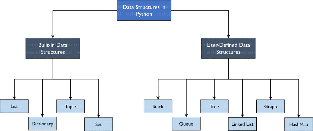
A data structure is a group of data elements grouped together under one name. Python’s data structures are very intuitive from a syntax point of view, and they offer a large choice of operations. This chapter tries to put together the most common and useful information about various data structures. Some of the Python’s data structures that are discussed in this book are list, tuple, set, and dictionary.

Types of Data Structures in Python
Python has implicit support for Data Structures which enable you to store and access data. These structures are called List, Dictionary, Tuple and Set.

Python allows its users to create their own Data Structures enabling them to have full control over their functionality. The most prominent Data Structures are Stack, Queue, Tree, Linked List and so on which are also available to you in other programming languages. So now that you know what are the types available to you, why don’t we move ahead to the Data Structures and implement them using Python.

TreeStructure-Data-Structures-in-Python

Built-in Data Structures
As the name suggests, these Data Structures are built-in with Python which makes programming easier and helps programmers use them to obtain solutions faster. Let’s discuss each of them in detail.

Python Programming – Data Structures Read More »

Python Programming – Tuple

In this Page, We are Providing Python Programming – Tuple. Students can visit for more Detail and Explanation of Python Handwritten Notes Pdf.

Python Programming – Tuple

Tuple

There is also another sequence type- tuple. Tuples is a sequence just like list. The differences are that tuple cannot be changed i.e. tuple is immutable, while list is mutable, and tuple use parentheses, while list use square brackets. Tuple items need not to be of same data type. Also, as mentioned previously, Python allow adding a trailing comma after last item of tuple.

>>> a= ( ' spam ' , ' eggs ' , 100 , 1234 )
>>> a
( ' spam ' , ' eggs ' , 100 , 1234 )
>>> a= ( ' spam ' , ' eggs ' , 100 , 1234 , )
>>> a
( ' spam ' , ' eggs ' , 100 , 1234 )

The above expressions are examples of a “tuple packing” operation i.e. the values ‘ spam ‘, ‘ eggs ‘, 10 0, and 123 4 are packed together in a tuple. The reverse operation is also possible, for example:

>>> a1 , a2 , a3 , a4=a 
>>> a1
' spam '
>>> a2 ' eggs '
>>> a3 100
>>> a4 1234

This is called “sequence unpacking”, and works for any sequence on the right-hand side. Sequence unpacking requires the group of variables on the left to have the same number of elements as the length of the sequence. Note that multiple assignments are really just a combination of tuple packing and sequence unpacking.

>>> a , b=10 , 20 
>>> a 
10
>>> b 
20

Tuple creation

Tuple can be created in many ways.

Using parenthesis

Creating a tuple is as simple as grouping various comma-separated-values, and optionally these comma-separated values between parentheses.

>>> a= ( ' spam ' eggs ' 100 , 1234 )
>>> a
( ' spam ' , ' eggs ' , 100 , 1234 )
>>> a= ( ' spam ' , ' eggs ' , 100 , 1234 )
>>> a
( ' spam ' , ' eggs ' , 100 , 1234 )
>>> a= ' spam ' , ' eggs ' , 100 , 1234 
>>> a
( ' spam ' , ' eggs ' , 100 , 1234 )
>>> a= ' spam ' , ' eggs ' , 100 , 1234 ,
>>> a
( ' spam ' , ' eggs ' , 100 , 1234 )

A tuple with one item is created by a comma after the item (it is not necessary to enclose a single item in parentheses).

>>> a= ( 10 )
>>> a 
10
>>> type ( a )
<type ' int ' >
>>> b= ( 10 ,)
>>> b
( 10 , )
>>> type ( b )
<type ' tuple ' >
>>> c=10,
>>> c
( 10 , )
>>> type ( c )
<type ' tuple ' >

It is also possible to create an empty tuple by assigning parenthesis to a variable.

>>> a= ( ) 
>>> a
( )

Using other tuples

A tuple can also be created by copying a tuple or slicing a tuple.

>>> a= ( ' spam ' , ' eggs ' , 100 , 1234 )
>>> b=a [ : ]
>>> b
( ' spam ' , ' eggs ' , 100 , 1234 )
>>> c=a [ 1 : 3 ]
>>> c
( ' eggs ' , 100 )

Using built-in function

Tuple can also be created using the built-in function tuple ( ). The tuple ( [iterable] ) function return a tuple whose items are the same and in the same order as items of the iterable. The iterable may be a sequence, a container that supports iteration, or an iterator object. If iterable is already a tuple, it is returned unchanged. If no argument is given, an empty tuple is returned.

>>> tuple ( [ ' apple ' , ' pineapple ' , ' banana ' ] )
( ' apple ' , ' pineapple ' , ' banana ' )
>>> tuple ( ' apple ' )
( ' a ' , ' p ' , ’ p ' , ’ 1 ’ , ’ e ’ )
>>> tuple ( [ ' apple ' ] ) 
( ' apple ' , )

Accessing tuple elements

The tuple index starts with 0, and to access values in a tuple, use the square brackets with the index or indices to obtain a slice of the tuple.

>>> a= ( ' spam ' , ' eggs ' , 100 , 1234 )
>>> a[ 0 ]
' spam '
>>> a [ 1 : 3 ]
( ' eggs ' , 100 )

Update tuple

Tuple is immutable, so changing element value or adding new elements is not possible. But one can take portions of existing tuples to create a new tuples.

>>> tuple1= ( 1 , 2 , 3 )
>>> tuple2=( ' a ' , ' b ' , ' c ' )
>>> tuple3=tuple1+tuple2 
>>> tuple3
( 1 , 2 , 3 , ' a ' , ' b ' , ' c ' )
>>> tuple3=tuple1 [ 0 : 2 ]+tuple2 [ 1 : 3 ] 
>>> tuple3
( 1 , 2 , ' b ' , ' c ' )

It is also possible to create tuple which contain mutable objects, such as lists.

>>> a= [ 1 , 2 , 3 ] , [ 4 , 5 , 6 , 7 ]
>>> a
( [ 1 , 2 , 3 ] , [ 4 , 5 , 6 , 7 ] )
>>> a [ 0 ] [ 1 ]=200
>>> a 
( [ 1 , 200 , 3 ] , [ 4 , 5 , 6 , 7 ] )

Deleting tuple

Removing individual tuple elements is not possible. To explicitly remove an entire tuple, just use the del statement.

>>> a= ( ' spam ' ' eggs ' , 100 , 1234 )
>>> del a

Swapping tuples

There might be a scenario in which multiple tuples needs to be swapped among themselves. This is can done easily using multiple assignments expression.

>>> a= ( 10 , 20 , 30 )
>>> b= ( 40 , 50 , 60 )
>> c= ( 70 , 80 , 90 )
>>> a , b , c=c , a , b 
>>> a
( 70 , 80 , 90 )
>>> b
( 10 , 20 , 30 )
>>> c
( 40 , 50 , 60 )

Python Programming – Tuple Read More »

Python Programming – Some List Operations

In this Page, We are Providing Python Programming – Some List Operations. Students can visit for more Detail and Explanation of Python Handwritten Notes Pdf.

Python Programming – Some List Operations

Some list operations

Some of the list operations supported by Python are given below.

Concatenation

List concatenation can be carried out using the + operator.

>>> [ 1 , 2 , 3 ] +[ ' hi ' , ' hello ' ]
[ 1 , 2 , 3 , ' hi ' , ' hello ' ] ;

Repetition

The * operator can be used to carry out repetition operations.

>>> [ ' Hey ' ] *3 
[ ' Hey ' , ' Hey ' , ' Hey ' ]

Membership operation

The list also supports membership operation i.e. checking the existence of an element in a list.

>>> 4 in [ 6 , 8 , 1 , 3 , 5 , 0 ]
False 
>>> 1 in [ 6 , 8 , 1 , 3 , 5 , 0 ]
True

Slicing operation

As list is a sequence, so indexing and slicing work the same way for list as they do for strings. All slice operations return a new list containing the requested elements:

>>> a= [ ' spam ' , ' eggs ' , 100 , 1234 ]
>>> a [ 2 ] 
100
>>> a [ -2 ]
100
>>> a [ 1 : 3 ] 
[ ' eggs ' , 100 ]
>>> a [ : ]
[ ' spam ' , ' eggs ' , 100 , 1234 ]

List slicing can be in form of steps, the operation s [ i: j: k ] slices the list s from i to j with step k.

>>> squares=[ x**2 for x in range ( 10 ) ] 
>>> squares
[ 0 , 1 , 4 , 9 , 16 , 25 , 36 , 49 , 64 , 81 , 100 , 121 , 144 , 169 , 196 ]
>>> squares [ 2 : 12 : 3 ]
[ 4 , 25 , 64 , 121 ]

Slice indices have useful defaults, an omitted first index defaults to zero, an omitted second index defaults to the size of the list being sliced.

>>> squares= [ x**2 for x in range ( 10 ) ]
>>> squares 
[0 , 1 , 4 , 9 , 16 , 25 , 36 , 49 , 64 , 81 , 100 , 121 , 144 , 169 , 196 ]
>>> squares [ 5 : ]
[ 25 , 36 , 49 , 64 , 81 , 100 , 121 , 144 , 169 , 196 ]
>>> squares [ : 5 ]
[ 0 , 1 , 4 , 9 , 16 ]

Python Programming – Some List Operations Read More »

Python Programming – Modules and Packages

In this Page, We are Providing Python Programming – Modules and Packages. Students can visit for more Detail and Explanation of Python Handwritten Notes Pdf.

Python Programming – Modules and Packages

As the program gets longer, it is a good option to split it into several files for easier maintenance. There might also be a situation when the programmer wants to use a handy function that is used in several programs without copying its definition into each program. To support such scenarios, Python has a way to put definitions in a file and use them in a script or in an interactive instance of the interpreter.

Module

A module is a file containing Python definitions and statements. The file name is the module name with the suffix .py appended. Definitions from a module can be imported into other modules. For instance, consider a script file called “fibo.py” in the current directory with the following code.

# Fibonacci numbers module

def fib ( n ) :                                        # write Fibonacci series up to n
         a , b=0 , 1 
         while b<n :
            print b , 
            a, b=b , a+b

def fib2 ( n ) :                                    # return Fibonacci series up to n
          result= [ ] 
          a , b = 0 , 1 
          while b<n:
               result . append ( b ) 
          a , b=b , a+b 
   return result

Now on the Python interpreter, import this module with the following command:

>>> import fibo

Within a module, the module’s name (as a string) is available as the value of the global variable
___name___:

>>> fibo.___name___ 
' fibo '

Use the module’s name to access its functions:

>>> fibo . fib ( 1000 )
1 1 2 3 5 8  13  21  34  55  89  144  233  377  610  987 
>>> fibo . fib2 ( 1000 )
[ 1 ,  1 ,  2 ,  3 ,  5 ,  8 ,  13 ,  21 ,  34 ,  55 ,  89 ,  144 ,  233 ,  377 ,  610 ,  987 ]

If it is intended to use a function often, assign it to a local name:

>>> Fibonacci=fibo . fib 
>>> Fibonacci ( 500 )
1  1  2  3  5  8  13  21  34  55  89  144  233  377

Python Programming – Modules and Packages Read More »

Python Programming – Modules

In this Page, We are Providing Python Programming – Modules. Students can visit for more Detail and Explanation of Python Handwritten Notes Pdf.

Python Programming – Modules

Modules

A module can contain executable statements as well as function definitions. These statements are intended to initialize the module. They are executed only the first time the module name is encountered in an import statement; they also run if the file is executed as a script.

Each module has its own private symbol table, which is used as the global symbol table by all functions defined in the module. Thus, the author of a module can use global variables in the module without worrying about accidental clashes with a user’s global variables.

Modules can import other modules. It is customary but not required to place all import statements at the beginning of a module. The imported module names are placed in the importing module’s global symbol table.

There is a variant of the import statement that imports specific names from a module directly into the importing module’s symbol table. For example, specific attributes of fibo module are imported in the local namespace as:

>>> from fibo import fib, fib2 
>>> fib ( 500 )
1 1 2 3 5 8 13 21 34 55 89 144 233 377

This does not introduce the module name from which the imports are taken in the local symbol table (so in the example, fibo is not defined).

There is even a variant to import all names that a module defines:

>>> from fibo import *
>>> fib ( 500 )
1 1 2 3 5 8 13 21 34 55 89 144 233 377

This imports all names except those beginning with an underscore ( _ ).

Note that in general, the practice of importing * from a module or package is discouraged, since it often causes poorly readable code. However, it is touse it to save typing in an interactive sessions. For efficiency reasons, each module is only imported once per interpreter session. If changes are made in many modules, it is a wise approach to restart the interpreter or if it is just one module that needs to be tested interactively, use reload (), e.g. reload (modulename).

Executing modules as scripts

When a Python module is run at command prompt

$ python fibo . py <arguments>

the code in the module will be executed, just as if it imported, but with the ___name___ set to ___main___ . That means, by adding the following code at the end of the module:

if __name___ == " ___main___ " :
import sys
fib ( int ( sys . argv [ 1 ] ) )

the file is made usable as a script as well as an importable module, because the code that parses the command line only runs if the module is executed as the “main” file:

$ python fibo . py 50 
1 1 2 3 5 8 13 21 34

The Module Search Path

When a module named f ibo is imported, the interpreter first searches for a built-in module with that name. If not found, it then searches for a file named fibo.py in a list of directories given by the variable sys. path. The variable sys. the path is initialized from some of these locations:

  • The current directory.
  • PYTHONPATH environment variable (a list of directory names, with the same syntax as the shell variable PATH).

After initialization, Python programs can modify sys .path. The directory containing the script being run is placed at the beginning of the search path, ahead of the standard library path. This means that scripts in that directory will be loaded instead of modules of the same name in the library directory.

Math module

Python has math module and it is always available. The functions provided in this module cannot be used with complex numbers; use the functions of the same name from the cmath module for support of complex numbers. The distinction between functions which support complex numbers and those which does not is made since most users do not want to learn quite as much mathematics as required to understand complex numbers. Except when explicitly noted otherwise, all functions return float values.

Python Programming – Modules Read More »